PID control algorithm learning

This article is reproduced from: Original link，Original author.
Here is just to record your learning process and add some simple code comments to complete it.

1. Where is PID algorithm used?

PID: proportion, integral, differential
PID algorithm can be used to control temperature, pressure, flow, chemical composition, speed and so on. Constant speed cruise of automobile; Speed position control in servo driver; Temperature of cooling system; The pressure of the hydraulic system can be realized by PID algorithm to ensure the stability of the system.

2. Principle of PID algorithm

First understand several concepts:

Deviation / error e: the difference between the output and target of the system at a certain time

parameter	Corresponding concept
K p K_p Kp​	Scale factor
K i K_i Ki​	Integral coefficient
K d K_d Kd​	Differential coefficient
T i T_i Ti​	Integration time
T d T_d Td​	Differential time

schematic diagram

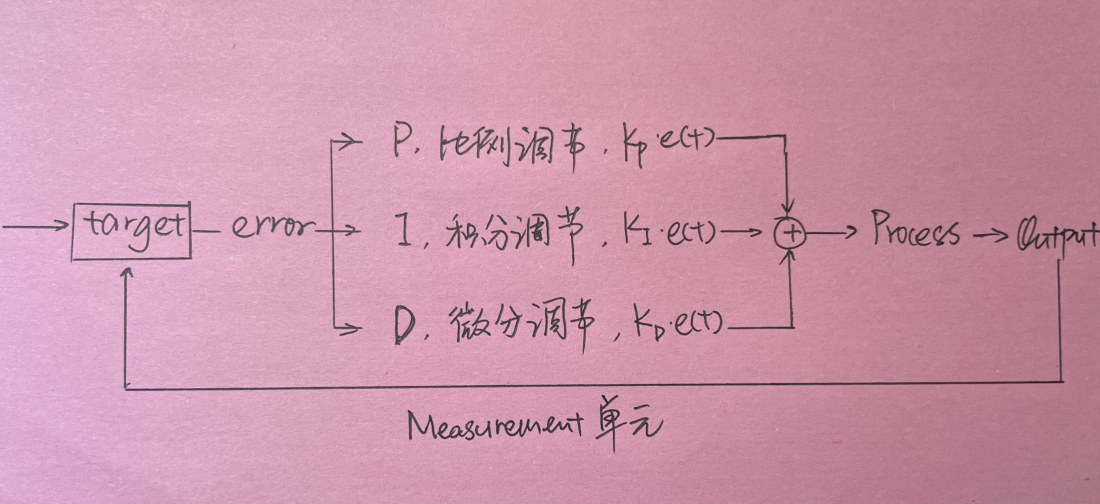
As shown in the figure, when the output is obtained, the difference between the output and the input is taken as the deviation, and the deviation signal is added to the input in a certain way after being superimposed through three operation modes of proportion, integration and differentiation, so as to control the final result and achieve the desired output value.

formula

PID formula principle:

y ( t ) = K p e ( t ) + 1 T i ∫ e ( t ) d t + T d d e ( t ) d t y(t) = K_pe(t) + {1\over T_{i}} \int e(t)dt + T_d {d e(t) \over dt} y(t)=Kp​e(t)+Ti​1​∫e(t)dt+Td​dtde(t)​

If it needs to be implemented on a computer, it needs to be discretized:

u [ k ] = K p e [ k ] + K i ∑ n = 0 k e [ n ] + K d ( e [ k ] − e [ k − 1 ] ) u[k] = K_p e[k] + K_i \sum_{n=0}^k e[n] + K_d(e[k]-e[k-1]) u[k]=Kp​e[k]+Ki​∑n=0k​e[n]+Kd​(e[k]−e[k−1])

( N o t e   t h a t :   T T i = K i ,   T T d = K d ) (Note \ that: \ {T \over T_i} = K_i, \ {T \over T_d} = K_d) (Note that: Ti​T​=Ki​, Td​T​=Kd​)

Scale factor K p K_p Kp​:

Increasing the scale coefficient makes the system sensitive, the adjustment speed is accelerated, and the steady-state error can be reduced. However, if the proportional coefficient is too large, the overshoot will increase, the oscillation times will increase, the adjustment time will be prolonged, the dynamic performance will deteriorate, and if the proportional coefficient is too large, the closed-loop system will even be unstable.

Proportional control cannot eliminate steady-state error.

Integral coefficient K i K_i Ki​:

The system eliminates the steady-state error and improves the error free degree. The function of integral control is that as long as there is error in the system, the integral adjustment will be carried out, the integral controller will continuously accumulate and output the control quantity until there is no error, the integral adjustment will stop, and the integral adjustment will output a constant value. Therefore, as long as there is enough time, the integral control will completely eliminate the error and make the system error zero, so as to eliminate the steady-state error. The strength of the integration action depends on the integration time constant ti. The smaller Ti, the stronger the integration action. Too strong integration action will increase the system overshoot and even cause the system to oscillate. On the contrary, if ti is large, the integration action is weak. Adding integral adjustment can reduce the stability of the system and slow down the dynamic response.

Differential coefficient K d K_d Kd​:

Differential control can reduce overshoot, overcome oscillation, improve the stability of the system, accelerate the dynamic response speed of the system and reduce the adjustment time, so as to improve the dynamic performance of the system.

The control effect of differential is related to the change speed of deviation. Differential control can predict deviation, produce advanced correction effect and help to reduce overshoot.

3. python implementation of PID algorithm

Firstly, a PID algorithm module is established. The algorithm principle is the above formula, which is saved as PID Py, as follows:

import time

class PID:
    def __init__(self, P, I, D):
    　　# Input coefficient
        self.Kp = P
        self.Ki = I
        self.Kd = D
        self.sample_time = 0.00
        self.current_time = time.time()
        self.last_time = self.current_time
        self.clear()
    def clear(self):
        self.SetPoint = 0.0	# True expectation 0.0
        self.PTerm = 0.0
        self.ITerm = 0.0
        self.DTerm = 0.0
        self.last_error = 0.0
        self.int_error = 0.0
        self.output = 0.0
    def update(self, feedback_value):
        # Calculation error - real error
        error = self.SetPoint - feedback_value
        # Calculate elapsed time (differential time) - delta t
        self.current_time = time.time()
        delta_time = self.current_time - self.last_time
        # Variation of calculation error (differential error) - delta e
        delta_error = error - self.last_error
        if (delta_time >= self.sample_time):
            self.PTerm = self.Kp * error # Scale factor term
            self.ITerm += error * delta_time # Integral coefficient term
            self.DTerm = 0.0
            if delta_time > 0:
                self.DTerm = delta_error / delta_time # Differential coefficient term
            self.last_time = self.current_time # Record new time node
            self.last_error = error # Record new error
            self.output = self.PTerm + (self.Ki * self.ITerm) + (self.Kd * self.DTerm)


    def setSampleTime(self, sample_time):
        self.sample_time = sample_time

Then create a test under the same path_ pid. Py, the algorithm diagram of realizing PID control is as follows:

import PID #Import the above PID algorithm
import time
import matplotlib.pyplot as plt
import numpy as np
from scipy.interpolate import make_interp_spline


def test_pid(P, I , D, L):
	# Initialize instance
    pid = PID.PID(P, I, D)
	
	# True expectation 1.1
    pid.SetPoint=1.1
    # Start sampling time. 01
    pid.setSampleTime(0.01)
	
	# Number of samples
    END = L
    feedback = 0
    feedback_list = []
    time_list = []
    setpoint_list = []

    for i in range(1, END):
        pid.update(feedback)
        output = pid.output
        feedback += output # Function of PID control system - correction value returned
        time.sleep(0.01)
        feedback_list.append(feedback) # Record the output value after each PID algorithm adjustment
        setpoint_list.append(pid.SetPoint)
        time_list.append(i)

	# Drawing part
    time_sm = np.array(time_list)
    time_smooth = np.linspace(time_sm.min(), time_sm.max(), 300)
    # Interpolation - draw smooth curves for better display
    feedback_smooth = make_interp_spline(time_list, feedback_list)(time_smooth)
    plt.figure(0)
    plt.grid(True)
    plt.plot(time_smooth, feedback_smooth,'b-')
    plt.plot(time_list, setpoint_list,'r')
    plt.xlim((0, L))
    plt.ylim((min(feedback_list)-0.5, max(feedback_list)+0.5))
    plt.xlabel('time (s)')
    plt.ylabel('PID (PV)')
    plt.title('PythonTEST PID--xiaomokuaipao',fontsize=15)

    plt.ylim((1-0.5, 1+0.5))

    plt.grid(True)
    plt.show()

if __name__ == "__main__":
    test_pid(1.2, 1, 0.001, L=100)

The final output is as follows:

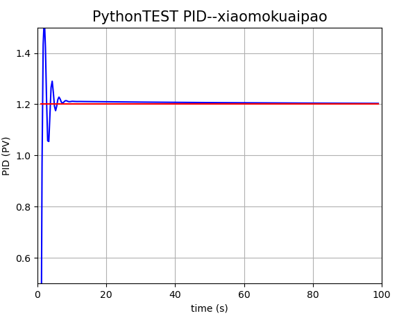
Among them, the red line is the target value (setpoint), and the blue line is the current value K p K_p Kp​， K i K_i Ki​， K d K_d The oscillation result under Kd} parameter finally tends to the target value and realizes the control.

Thus, the simple schematic of PID algorithm is realized in python.

4. Some experience in PID debugging

General principles of PID commissioning:

When the output is not oscillatory, increase the proportional gain;

Reduce the integral time constant when the output is not oscillatory;

When the output is not oscillatory, increase the differential time constant;

PID regulation formula:

Find the best parameter setting, and check from small to large in sequence

First proportional, then integral, and finally add differential

The curve oscillates frequently, and the scale dial should be enlarged

The curve floats around the big bay, and the scale dial pulls to the small

The curve deviates and recovers slowly, and the integration time decreases

The curve has a long fluctuation period and the integration time is longer

The oscillation frequency of the curve is fast. First reduce the differential

The fluctuation is slow due to large dynamic difference, and the differential time should be prolonged

The ideal curve has two waves, the front is higher and the back is lower by four to one

One look, two adjustments and more analysis, the adjustment quality will not be low