Teacher Wu began to build a hidden neural network.
1, Importing datasets and drawing
Two files are required before importing the dataset. Please refer to [data]
import numpy as np
import pandas as pd
from matplotlib import pyplot as plot
from testCases import *
import sklearn
from sklearn import datasets
from sklearn import linear_model
from planar_utils import *
plt.rcParams['font.sans-serif']=['SimHei'] #Used to display Chinese labels normally
plt.rcParams['axes.unicode_minus']=False #Used to display negative signs normally
np.set_printoptions(suppress=True)#Prevent scientific counting

np.random.seed(1)
X,Y = load_planar_dataset()
plt.figure(figsize=(12,8))
plt.scatter(X[0,:],X[1,:],c = Y.flatten(),label = 'Scatter')
plt.show()
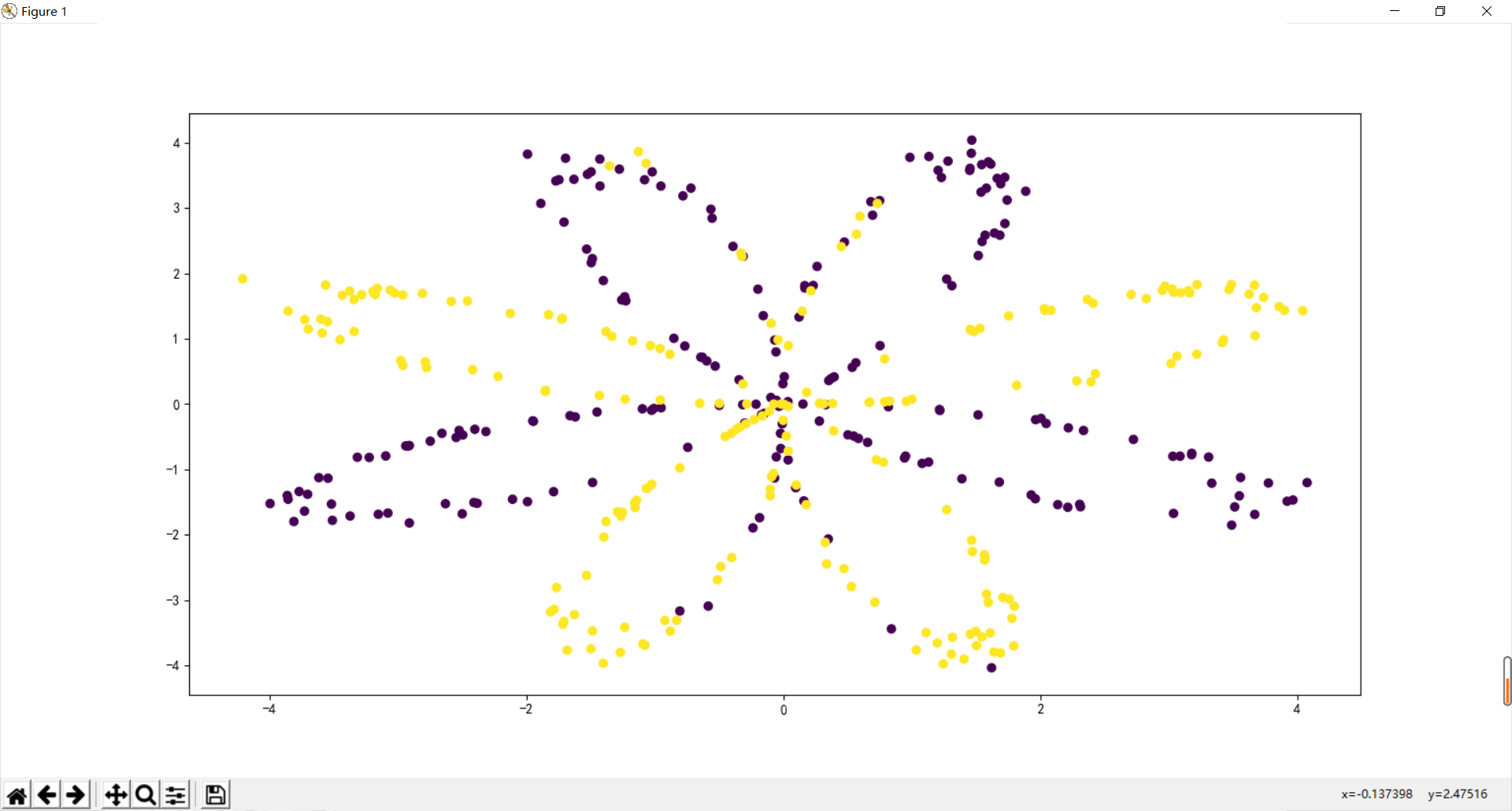
In PLT The parameter c in scatter () is color, which is assigned as an iteratable parameter object with the same length as X and Y. according to the different values, the (x,y) parameter pairs show different colors. Simply put, it's good to distinguish colors according to one of the X and Y values. For example, the upper side wants to distinguish colors according to the y value, so it's OK to directly c=y.
2, logistic regression test
Instead of building wheels like the previous machine learning, directly call the sklearn function and test it with logistic regression.
# 10: All sample dimensions are 2 * 400
# Y: All label dimensions are 1 * 400 (0 | 1)
lr = linear_model.LogisticRegression()
lr.fit(X.T,Y.flatten())
#View its corresponding w
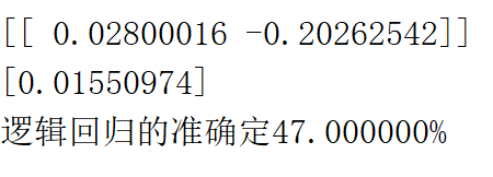
print(lr.coef_)
#View its corresponding w0
print(lr.intercept_)
w1 = lr.coef_[0,0]
w2 = lr.coef_[0,1]
w0 = lr.intercept_
c = np.linspace(min(X[0,:]),max(X[0,:]),100)
f = [(-w1*i-w0)/w2 for i in c]
plt.plot(c,f,label = 'Classification curve',color = 'r')
plt.legend()
plt.show()
#An array of prediction results
res = lr.predict(X.T)
print('Quasi determination of logistic regression%f%%'%((float(np.dot(Y,res))+float(np.dot(1-Y,1-res)))/Y.size*100)) 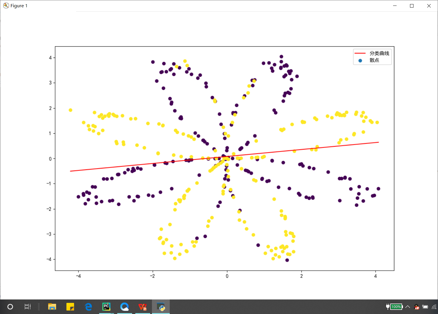
The drawing method I just used is different from that of Mr. Wu. He also specially wrote a function to draw the classification line. I drew it directly by using W0, W1 and W2, because w0+w1*x1+w2*x2 = 0, which is just a function and can roughly draw the effect of Mr. Wu.
I wanted to use this linear function to draw a closed circle before. I tried it many times, but I still didn't draw it. Later, I thought, this itself is a primary function. How can I draw the image of a quadratic function?
3, Build neural network model
General methods of constructing neural networks:
1. Define the structure of neural network
2. Analyze the dimensions of the corresponding parameters of each layer structure
3. Define activation function
4. Initialize model parameters
5. Define forward propagation function
6. Calculate loss
7. Define back propagation function
8. Iterative integration
9. Forecast
10. Image analysis
The network model is as follows:
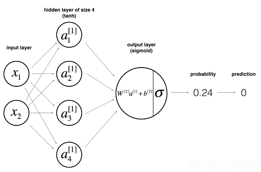
According to the model picture, calculate the dimension of the parameter (speculate a little, so as to facilitate vector multiplication with np later):
X: 2 * 400 * dataset x is a total of 400, with 2 features each
Y: Classification of each sample (1240 * 1)
The W dimension of the first layer is 4 * 2, because there are four nodes in this layer and two nodes in the previous layer
B of the first layer: because this layer has 4 nodes, it is 4 * 1
Therefore, Z and A of the first layer are 4 * 400 , because there are 400 samples , and the activation function is tanh
The W dimension of the second layer is 1 * 4. This layer has one node and the upper layer has four nodes, which is similar to logistic regression
B in the second layer: dimension 1 * 1 is a single value
Z and A of the second layer: 1 * 400 ^ the activation function is sigmoid
4, Define model structure
Defining the structure of the model is mainly to define the quantity contained in each layer, and also to define the sigmoid function. For the tanh function, you can use NP Tanh()
def sigmoid(x):
    return 1/(1+np.exp(-x))


def layer_size(X,Y):
    #Input layer
    n_x = X.shape[0]
    #Hidden layer
    n_h = 4
    #Output layer
    n_y = Y.shape[0]
    return n_x,n_h,n_y
I think because there are few layers in this model, if there are many layers, an array may be used to store the corresponding number of each layer.
5, Initialize w and b
It can be seen from the model that this is a two-layer model, so it needs two layers to measure W and B
For W: use random values to initialize the matrix. It is not possible to set the initial w to all 0 matrices like logistic
w1 = np.random.randn(n_h,n_x)*0.01
For b: it can be set to all 0 matrix
b1 = np.zeros((n_h,1))
def initialize_parameters(n_x,n_h,n_y):
    '''
    It is determined according to the number of each layer. Because this is a two-layer model, the first layer needs to be defined W and B Second floor W and B
    :param n_x:
    :param n_h:
    :param n_y:
    :return:
    '''
    np.random.seed(2)
    w1 = np.random.randn(n_h,n_x)*0.01
    b1 = np.zeros((n_h,1))
    w2 = np.random.randn(n_y,n_h)*0.01
    b2 = np.zeros((n_y,1))

    parameters = {
        'w1':w1,
        'w2': w2,
        'b1': b1,
        'b2': b2,
    }

    return parameters
np.random.seed(2), like the number generated by the teacher, I have to say that the boss is considerate, which is convenient to verify the correctness of our experiment.
6, Forward propagation
def forward_propagation(X,parameters):
    '''
    Realize forward propagation
    :param X:Sample matrix 2*400
    :param parameters:  Initialized w and b Dictionary of composition
    :return:
    '''
    w1 = parameters['w1']#4*2
    b1 = parameters['b1']#4*1
    w2 = parameters['w2']#1*4
    b2 = parameters['b2']#1*1

    Z1 = np.dot(w1,X)+b1#4*400
    A1 = np.tanh(Z1)#4*400
    Z2 = np.dot(w2,A1)+b2#1*400
    A2 = sigmoid(Z2)#1*400

    cache = {
        "Z1":Z1,
        "A1": A1,
        "Z2": Z2,
        "A2": A2
    }

    return A2,cache
When writing code, it is best to think about the dimension of the matrix generated at each step and observe whether the form of (1, m) can be generated at the end.
VII. Cost function
After the forward propagation is completed, the cost function must be calculated. The code is as follows:
def compute_cost(A2,Y):
m = Y.shape[1]
first = np.multiply(-Y,np.log(A2))
second = np.multiply(1-Y,np.log(1-A2))
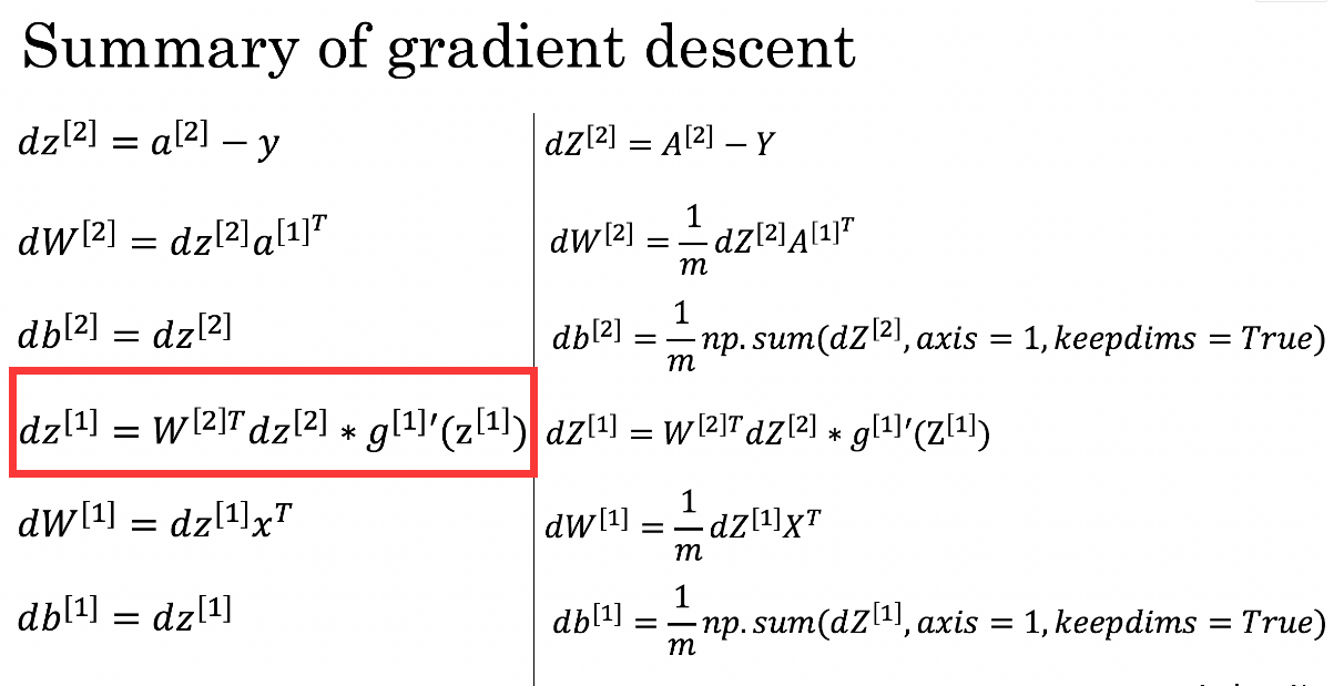
return np.sum(first-second)/m8, Back propagation
I think this is the most difficult part. The reason why I think it is difficult is that I still haven't deduced these formulas up to now. I will deduce the single-layer neural network, but once the hidden layer is added, the step containing the derivative of the activation formula is not deduced. Take your time and discuss with others.
def backward_propagation(parameters,cache,X,Y):
    '''

    :param parameters: Contains w1 w2 b1 b2
    :param cache: Contains Z1 Z2 A1 A2
    :param X: input data
    :param Y: label
    :return: grads Dictionary contains dw and db
    '''

    #X;2*400
    #Y;1*400

    m = X.shape[1]
    w1 = parameters['w1']#4*2
    w2 = parameters['w2']#1*4

    A1 = cache['A1']#4*400
    A2 = cache['A2']#1*400

    dz2 = A2-Y#1*400
    dw2 = (1/m)*np.dot(dz2,A1.T)#1*4
    db2 = (1/m)*np.sum(dz2,axis = 1,keepdims = True)#1*1
    #The hardest part to understand
    dz1 = np.multiply(np.dot(w2.T,dz2),1-np.power(A1,2))#4*400
    dw1 = (1/m)*np.dot(dz1,X.T)#4*2
    db1 = (1/m)*np.sum(dz1,axis = 1,keepdims = True)#4*1

    grads = {
        'dw1':dw1,
        'db1': db1,
        'dw2': dw2,
        'db2': db2,
    }
    return grads
9, Iterative update parameters
Perform gradient descent and update iteration on the parameters obtained above
def update_parameters(parameters,grads,learning_rate = 1.2):
    '''
    to update w1  w2  b1 b2
    :param parameters:
    :param grads:
    :param learning_rate:
    :return:
    '''

    w1 = parameters['w1']
    w2 = parameters['w2']
    b1 = parameters['b1']
    b2 = parameters['b2']

    dw2 = grads['dw2']
    dw1 = grads['dw1']
    db2 = grads['db2']
    db1 = grads['db1']

    w2 = w2 - learning_rate*dw2
    b2 = b2 - learning_rate * db2
    w1 = w1 - learning_rate * dw1
    b1 = b1 - learning_rate * db1

    parameters = {
        'w1': w1,
        'w2': w2,
        'b1': b1,
        'b2': b2,
    }
    return parameters
10, Integration model
def nn_model(X,Y,n_h,num_iterations,print_cost=False):


    np.random.seed(3)
    n_x = layer_size(X,Y)[0]
    n_y = layer_size(X,Y)[2]

    parameters = initialize_parameters(n_x,n_h,n_y)
    w1 = parameters['w1']
    w2 = parameters['w2']
    b1 = parameters['b1']
    b2 = parameters['b2']


    for i in range(num_iterations):
        A2,cache = forward_propagation(X,parameters)
        cost = compute_cost(A2,Y)
        grads = backward_propagation(parameters,cache,X,Y)
        parameters = update_parameters(parameters,grads,learning_rate=0.5)

        if print_cost:
            if i%100==0:
                print("The first",i,"Secondary cycle,Cost is"+str(cost))
    return parameters
11, Prediction results
I have to say, this prediction function is really beautiful!
def predict(parameters,X):
    A2,cache = forward_propagation(X,parameters)
    predictions = np.round(A2)
    return predictions
Twelve, model operation
parameters = nn_model(X,Y,4,10000,True)
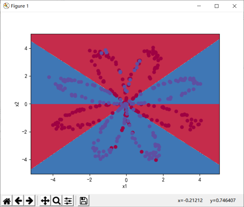
predictions = predict(parameters,X)
plot_decision_boundary(lambda x:predict(parameters,x.T),X,Y)
s1 = np.dot(Y,predictions.T)
s2 = np.dot(1-Y,1-predictions.T)
num = Y.size
print('Accuracy:%d%%'%float((s1+s2)/num*100))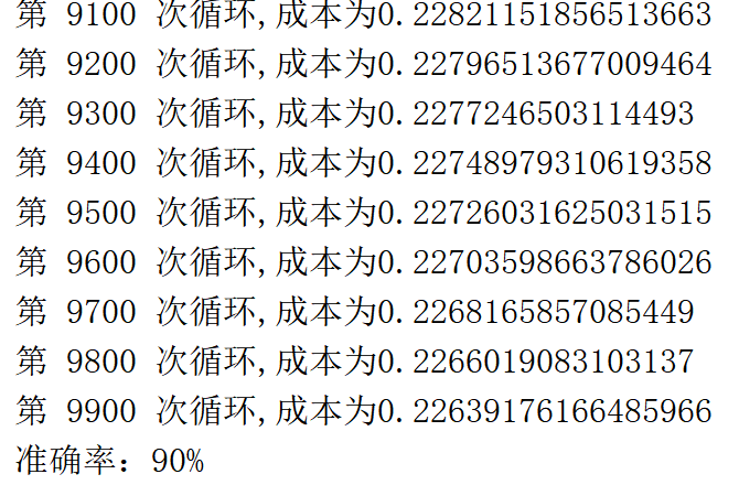
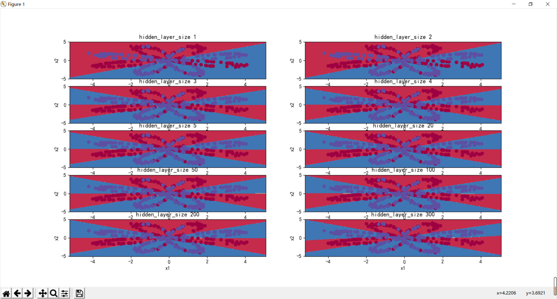
13, Different number of hidden layers
Use a for loop to observe the accuracy of different number of hidden layers
plt.figure(figsize=(16,32))
hidden_layer_sizes = [1,2,3,4,5,20,50,100,200,300]
for i,n_h in enumerate(hidden_layer_sizes):
    plt.subplot(5,2,i+1)
    plt.title('hidden_layer_size %d'%n_h)
    parameters = nn_model(X,Y,n_h,num_iterations=5000)
    plot_decision_boundary(lambda x: predict(parameters, x.T), X, Y)
    predictions = predict(parameters, X)
    s1 = np.dot(Y, predictions.T)
    s2 = np.dot(1 - Y, 1 - predictions.T)
    num = Y.size
    print('hidden_layer_size{}Accuracy:{}%%' .format(n_h,float((s1 + s2) / num * 100) ))

plt.show()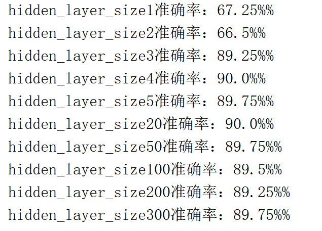
(after running it, I found that the accuracy rate was one% more, so I didn't modify it again)_ layer_ When the size is 4, it is best. In the previous operation, when the number of hidden layers is 5, it is only 90%, so the best scheme is 4 or 5 hidden layers (a little different from Mr. Wu's result), which is basically the same.
14, The activation function tanh becomes sigmoid
The specific code is to change the activation function and the derivative at the corresponding position.
The results are as follows:
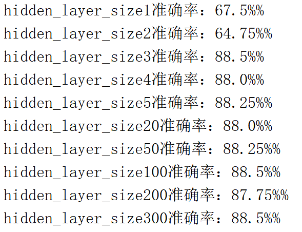
It can be seen that the overall result is not as good as the tanh activation function
15, Change learning rate
Forget to mention that all the above experimental results are generated when the number of iterations is 5000 and the learning rate is 0.5.
When the change learning rate is 0.1:
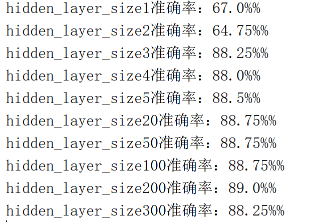
16, Summary
① : it can be seen from the above experimental summary that Mr. Wu has adjusted the code to the best
② : familiar with the construction of the whole neural network
③ : the line of code of the derivative in the back propagation is pondering
④ : after the model is built, the key is to adjust the super parameters to make w and b more appropriate
⑤ : continue to do teacher Wu's next experiment
17, Appendix code (do not use it directly)
import numpy as np
import pandas as pd
from matplotlib import pyplot as plot
from testCases import *
import sklearn
from sklearn import datasets
from sklearn import linear_model
from planar_utils import *
plt.rcParams['font.sans-serif']=['SimHei'] #Used to display Chinese labels normally
plt.rcParams['axes.unicode_minus']=False #Used to display negative signs normally
np.set_printoptions(suppress=True)#Prevent scientific counting


np.random.seed(1)

X,Y = load_planar_dataset()


#logistic regression
def logistic():
    plt.figure(figsize=(12,8))
    plt.scatter(X[0,:],X[1,:],c = Y.flatten(),label = 'Scatter')
    # 10: All sample dimensions are 2 * 400
    # Y: All label dimensions are 1 * 400 (0 | 1)
    lr = linear_model.LogisticRegression()
    lr.fit(X.T,Y.flatten())
    #View its corresponding w
    print(lr.coef_)
    #View its corresponding w0
    print(lr.intercept_)
    w1 = lr.coef_[0,0]
    w2 = lr.coef_[0,1]
    w0 = lr.intercept_

    c = np.linspace(min(X[0,:]),max(X[0,:]),100)
    f = [(-w1*i-w0)/w2 for i in c]
    plt.plot(c,f,label = 'Classification curve',color = 'r')
    plt.legend()
    plt.show()
    #An array of prediction results
    res = lr.predict(X.T)
    print('Quasi determination of logistic regression%f%%'%((float(np.dot(Y,res))+float(np.dot(1-Y,1-res)))/Y.size*100))


def sigmoid(x):
    return 1/(1+np.exp(-x))


def layer_size(X,Y):
    #Input layer
    n_x = X.shape[0]
    #Hidden layer
    n_h = 4
    #Output layer
    n_y = Y.shape[0]
    return n_x,n_h,n_y


def initialize_parameters(n_x,n_h,n_y):
    '''
    It is determined according to the number of each layer. Because this is a two-layer model, the first layer needs to be defined W and B Second floor W and B
    :param n_x:
    :param n_h:
    :param n_y:
    :return:
    '''
    np.random.seed(2)
    w1 = np.random.randn(n_h,n_x)*0.01
    b1 = np.zeros((n_h,1))
    w2 = np.random.randn(n_y,n_h)*0.01
    b2 = np.zeros((n_y,1))

    parameters = {
        'w1':w1,
        'w2': w2,
        'b1': b1,
        'b2': b2,
    }
    return parameters

def forward_propagation(X,parameters):
    '''
    Realize forward propagation
    :param X:Sample matrix 2*400
    :param parameters:  Initialized w and b Dictionary of composition
    :return:
    '''
    w1 = parameters['w1']#4*2
    b1 = parameters['b1']#4*1
    w2 = parameters['w2']#1*4
    b2 = parameters['b2']#1*1

    Z1 = np.dot(w1,X)+b1#4*400
    A1 = np.tanh(Z1)#4*400
    #A1 = sigmoid(Z1)
    Z2 = np.dot(w2,A1)+b2#1*400
    A2 = sigmoid(Z2)#1*400

    cache = {
        "Z1":Z1,
        "A1": A1,
        "Z2": Z2,
        "A2": A2
    }

    return A2,cache


def compute_cost(A2,Y):
    m = Y.shape[1]
    first = -np.multiply(Y,np.log(A2))
    second = np.multiply(1-Y,np.log(1-A2))

    return np.sum(first-second)/m


def backward_propagation(parameters,cache,X,Y):
    '''

    :param parameters: Contains w1 w2 b1 b2
    :param cache: Contains Z1 Z2 A1 A2
    :param X: input data
    :param Y: label
    :return: grads Dictionary contains dw and db
    '''

    #X;2*400
    #Y;1*400

    m = X.shape[1]
    w1 = parameters['w1']#4*2
    w2 = parameters['w2']#1*4

    A1 = cache['A1']#4*400
    A2 = cache['A2']#1*400

    dz2 = A2-Y#1*400
    dw2 = (1/m)*np.dot(dz2,A1.T)#1*4
    db2 = (1/m)*np.sum(dz2,axis = 1,keepdims = True)#1*1
    #The hardest part to understand
    dz1 = np.multiply(np.dot(w2.T,dz2),1-np.power(A1,2))#4*400
    #dz1 = np.multiply(np.dot(w2.T, dz2),A1*(1-A1) )  # 4*400
    dw1 = (1/m)*np.dot(dz1,X.T)#4*2
    db1 = (1/m)*np.sum(dz1,axis = 1,keepdims = True)#4*1

    grads = {
        'dw1':dw1,
        'db1': db1,
        'dw2': dw2,
        'db2': db2,
    }
    return grads


def update_parameters(parameters,grads,learning_rate = 1.2):
    '''
    to update w1  w2  b1 b2
    :param parameters:
    :param grads:
    :param learning_rate:
    :return:
    '''

    w1 = parameters['w1']
    w2 = parameters['w2']
    b1 = parameters['b1']
    b2 = parameters['b2']

    dw2 = grads['dw2']
    dw1 = grads['dw1']
    db2 = grads['db2']
    db1 = grads['db1']

    w2 = w2 - learning_rate*dw2
    b2 = b2 - learning_rate * db2
    w1 = w1 - learning_rate * dw1
    b1 = b1 - learning_rate * db1

    parameters = {
        'w1': w1,
        'w2': w2,
        'b1': b1,
        'b2': b2,
    }
    return parameters


def nn_model(X,Y,n_h,num_iterations,print_cost=False):


    np.random.seed(3)
    n_x = layer_size(X,Y)[0]
    n_y = layer_size(X,Y)[2]

    parameters = initialize_parameters(n_x,n_h,n_y)
    w1 = parameters['w1']
    w2 = parameters['w2']
    b1 = parameters['b1']
    b2 = parameters['b2']


    for i in range(num_iterations):
        A2,cache = forward_propagation(X,parameters)
        cost = compute_cost(A2,Y)
        grads = backward_propagation(parameters,cache,X,Y)
        parameters = update_parameters(parameters,grads,learning_rate=0.1)

        if print_cost:
            if i%100==0:
                print("The first",i,"Secondary cycle,Cost is"+str(cost))
    return parameters


def predict(parameters,X):
    A2,cache = forward_propagation(X,parameters)
    predictions = np.round(A2)
    return predictions


plt.figure(figsize=(16,32))
hidden_layer_sizes = [1,2,3,4,5,20,50,100,200,300]
for i,n_h in enumerate(hidden_layer_sizes):
    plt.subplot(5,2,i+1)
    plt.title('hidden_layer_size %d'%n_h)
    parameters = nn_model(X,Y,n_h,num_iterations=5000)
    plot_decision_boundary(lambda x: predict(parameters, x.T), X, Y)
    predictions = predict(parameters, X)
    s1 = np.dot(Y, predictions.T)
    s2 = np.dot(1 - Y, 1 - predictions.T)
    num = Y.size
    print('hidden_layer_size{}Accuracy:{}%%' .format(n_h,float((s1 + s2) / num * 100) ))

plt.show()