Continued [play yolov5] use TensorRT C++ API to build v4 Network structure (0) , the backbone part has been finished. Now let's move on to the neck part. Before continuing to explain the neck part, it is necessary to review PANet, because the neck part is an FPN+PAN structure.

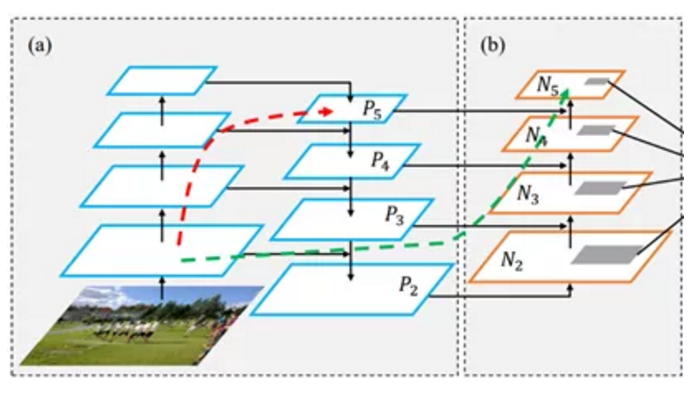
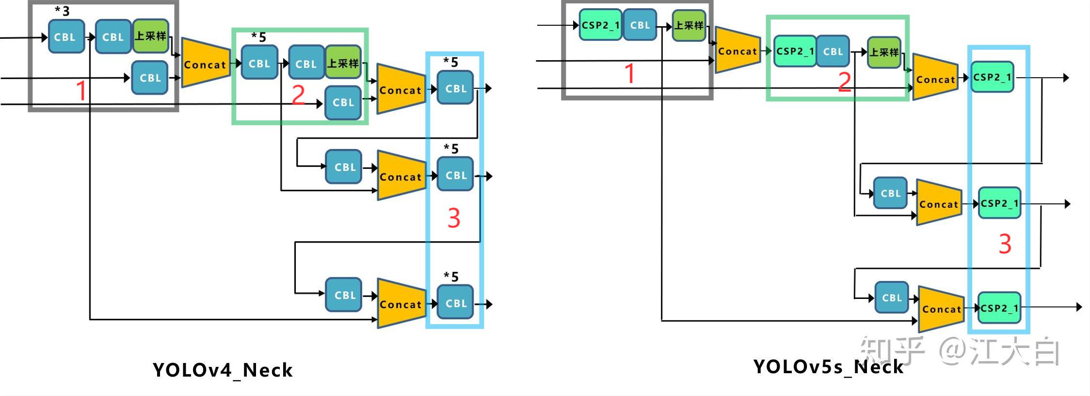
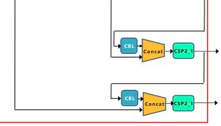
Based on FPN, PANet adds bottom up path augmentation, mainly considering that the shallow features of the network include a large number of edge shapes and other features, which play a vital role in the pixel level classification task of instance segmentation. The red arrow in the figure above indicates that in FPN, because it needs to go through a bottom-up process, the shallow features need to go through dozens or even up to the white layer network, and the shallow information is seriously lost. The red arrow indicates the bottom up path augmentation structure added by the author. This structure has less than ten layers. In this way, the shallow features are laterally connected to P2 through the original FPN, and then transferred from P2 to the top layer from Bottom-up Path Augmentation. The number of layers is small, which can better preserve the shallow features. Note that N2 and P2 here represent the same feature map, while N3, N4 and N5 are different from P3, P4 and P5. N3, N4 and N5 are the results of P3, P4 and P5 fusion. The Neck network of YOLOv5 still uses FPN+PAN structure, but some improved operations are made on its basis. The Neck structure of YOLOv4 adopts ordinary convolution operation. In the Neck network of YOLOv5, the CSP2 structure designed by CSPnet is used for reference, so as to strengthen the ability of network feature fusion. The following figure shows the specific details of the Neck networks of YOLOv4 and YOLOv5. Through comparison, we can find that: (1) the gray area represents the first difference, and YOLOv5 not only uses CSP2_1. The structure replaces some CBL modules and removes the lower CBL modules;

(2) The green area indicates the second difference. YOLOv5 not only replaces the CBL module after Concat operation with CSP2_1 module, and the position of another CBL module is replaced;

(3) The blue area indicates the third difference. YOLOv5 replaces the original CBL module with CSP2_1 module.

yolov5 contains three detection branches, which are on the characteristic graphs of 8x, 16 and 32x respectively. First, use tensort api to construct the Neck part of the first branch.

    auto bottleneck_csp9 = C3(network, weightMap, *spp8->getOutput(0), get_width(1024, gw), get_width(1024, gw), get_depth(3, gd), false, 1, 0.5, "model.9"); //CSP2_1
    auto conv10 = convBlock(network, weightMap, *bottleneck_csp9->getOutput(0), get_width(512, gw), 1, 1, 1, "model.10"); //CBL
    
    //The first upsampling, 32x - > upsample - > 16x
    auto upsample11 = network->addResize(*conv10->getOutput(0));
    assert(upsample11);
    upsample11->setResizeMode(ResizeMode::kNEAREST);
    upsample11->setOutputDimensions(bottleneck_csp6->getOutput(0)->getDimensions());

    //Concat
    ITensor* inputTensors12[] = { upsample11->getOutput(0), bottleneck_csp6->getOutput(0) };
    auto cat12 = network->addConcatenation(inputTensors12, 2);
    auto bottleneck_csp13 = C3(network, weightMap, *cat12->getOutput(0), get_width(1024, gw), get_width(512, gw), get_depth(3, gd), false, 1, 0.5, "model.13");
    auto conv14 = convBlock(network, weightMap, *bottleneck_csp13->getOutput(0), get_width(256, gw), 1, 1, 1, "model.14");
    
    //The second upsampling, 16x - > upsample - > 8x
    auto upsample15 = network->addResize(*conv14->getOutput(0));
    assert(upsample15);
    upsample15->setResizeMode(ResizeMode::kNEAREST);
    upsample15->setOutputDimensions(bottleneck_csp4->getOutput(0)->getDimensions());
	
    //Concat
    ITensor* inputTensors16[] = { upsample15->getOutput(0), bottleneck_csp4->getOutput(0) };
    auto cat16 = network->addConcatenation(inputTensors16, 2);
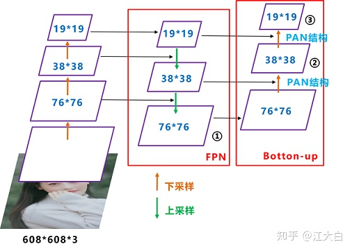
    auto bottleneck_csp17 = C3(network, weightMap, *cat16->getOutput(0), get_width(512, gw), get_width(256, gw), get_depth(3, gd), false, 1, 0.5, "model.17");

The CSP structure of Neck part is csp2_ 10. Csp2 was mentioned earlier_ X and csp1_ The most important difference of X is that some Bottleneck structures in the middle become ordinary convolution. The upper sampling part uses TensorRT API addResize(...) Function. After two up sampling operations, the 32x feature map is changed to 8x size.

Then construct the second and Third branches, which is relatively simple.

//The second branch
    auto conv18 = convBlock(network, weightMap, *bottleneck_csp17->getOutput(0), get_width(256, gw), 3, 2, 1, "model.18");
    ITensor* inputTensors19[] = { conv18->getOutput(0), conv14->getOutput(0) };
    auto cat19 = network->addConcatenation(inputTensors19, 2);
    auto bottleneck_csp20 = C3(network, weightMap, *cat19->getOutput(0), get_width(512, gw), get_width(512, gw), get_depth(3, gd), false, 1, 0.5, "model.20");
    IConvolutionLayer* det1 = network->addConvolutionNd(*bottleneck_csp20->getOutput(0), 3 * (Yolo::CLASS_NUM + 5), DimsHW{ 1, 1 }, weightMap["model.24.m.1.weight"], weightMap["model.24.m.1.bias"]);

    //The third branch
    auto conv21 = convBlock(network, weightMap, *bottleneck_csp20->getOutput(0), get_width(512, gw), 3, 2, 1, "model.21");
    ITensor* inputTensors22[] = { conv21->getOutput(0), conv10->getOutput(0) };
    auto cat22 = network->addConcatenation(inputTensors22, 2);
    auto bottleneck_csp23 = C3(network, weightMap, *cat22->getOutput(0), get_width(1024, gw), get_width(1024, gw), get_depth(3, gd), false, 1, 0.5, "model.23");
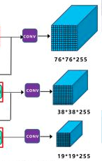
    IConvolutionLayer* det2 = network->addConvolutionNd(*bottleneck_csp23->getOutput(0), 3 * (Yolo::CLASS_NUM + 5), DimsHW{ 1, 1 }, weightMap["model.24.m.2.weight"], weightMap["model.24.m.2.bias"]);

The Head part of Yolov5 adopts 1x1 convolution structure, with a total of three groups of outputs. The size resolution of the output characteristic image is:

 

BS x 255 x 76 x76

BS x 255 x 38 x 38

BS x 255 x 19 x 19

Where BS is Batch Size, and the calculation method of 255 is [na * (nc + 1 + 4)]. Specific parameters

• Na (number of anchors) is the scale number of each group of anchors (there are 3 groups of anchors in YOLOv5, and each group has 3 scales);

• nc is number of class (coco's class is 80);

• 1 is the confidence score of foreground and background;

• 4 is the coordinate and width height of the center point;

Finally, the anchor box will be applied to the output feature map, and the final output vector with category probability, confidence score and bounding box will be generated.

    IConvolutionLayer* det0 = network->addConvolutionNd(*bottleneck_csp17->getOutput(0), 3 * (Yolo::CLASS_NUM + 5), DimsHW{ 1, 1 }, weightMap["model.24.m.0.weight"], weightMap["model.24.m.0.bias"]);
    IConvolutionLayer* det1 = network->addConvolutionNd(*bottleneck_csp20->getOutput(0), 3 * (Yolo::CLASS_NUM + 5), DimsHW{ 1, 1 }, weightMap["model.24.m.1.weight"], weightMap["model.24.m.1.bias"]);
    IConvolutionLayer* det2 = network->addConvolutionNd(*bottleneck_csp23->getOutput(0), 3 * (Yolo::CLASS_NUM + 5), DimsHW{ 1, 1 }, weightMap["model.24.m.2.weight"], weightMap["model.24.m.2.bias"]);

[References]

https://docs.nvidia.com/deeplearning/tensorrt/developer-guide/index.html#create_network_c #nvidia official