catalogue
2, Generation of data table (usually import data table)
3, Data table information viewing
2. Basic information of data table (dimension, column name, data format, occupied space, etc.)
3. View the format of each column of data
6. View a column of null values
7. View the unique value of a column
8. View the values in the data table
9. View the name of the column
10. View the first n rows of data and the last n rows of data
2. Fill NaN with the mean value of the column price:
3. Clear the character space in the city field
7. Duplicate values after / after deletion
3. Sort by the value of a specific column
6. Group and mark the data with multiple conditions
8. The split data sheet and the original DF will be completed_ Match the inner data table
1. Extract the value of a single line by index
2. Extract area row values by index
3. Reset Index & set other indexes & extract selected index data
4. Use iloc to extract data by location area
5. Adapt to iloc lifting data separately by location
6. Use ix to extract data by index label and location
7. Judge whether the value of city column is Beijing
9. Extract the first three characters and generate a data table
1. Use "and", "or" and "not" to filter
2. Count the filtered data by city column
3. Use the query function to filter
4. Sum the filtered results according to prince
1. Count and summarize all columns
3. Summarize and count the two fields
4. Summarize the city field and calculate the total and average value of prince respectively
1. Simple data sampling (random)
2. Manually set the sampling weight
3. Do not put it back after sampling
5. Descriptive statistics of data sheet
6. Calculate the standard deviation of the column
7. Calculate the covariance between the two fields
8. Covariance between all fields in the data table
9. Correlation analysis of two fields
10. Correlation analysis of data sheet
(^ - ^): Introduction
As we all know, it is very important to master data processing methods in the data age. Pandas is a very excellent and widely used third-party library in python. (I admit that those words are water words. I'm sorry to boast about konjak, but pandas is really a very easy-to-use library). Who knows the happiness of pandas [doge]. At least I've learned well~
It must be noted that as a konjac, the degradation article of pandas is not what I can write. After referring to the article of the big man, I do some nanny level explanations according to what I feel and understand when I study. (although there is detailed code in the big guy's article, there is no display of the running results, which is unfriendly to friends who are inconvenient to try to see the results. Many small details are completely unknown to beginners. They can only be understood by referring to the degradation of other small articles. This is a summary ~)
Big guy article link: pandas Usage Summary
The foreplay is very long. Thank you for watching it!

1, Installing pandas
General operation: open CMD (for Windows system, you can enter CMD in the search column in the lower left corner of the screen) and enter PIP install pandas (for Python 3, you can also change pip to pip3, which is no difference).
pip install pandas
Reference article: Installation of pandas
2, Generation of data table (usually import data table)
1. Import library
First, explain that pandas and numpy usually work together, so form the habit of importing numpy while importing pandas!
import numpy as np
import pandas as pd
About numpy, if you want to learn, my big brother roommate has a detailed article, which is linked here. Please feel free.
Python: the most basic knowledge of numpy module
2. Import file
df = pd.DataFrame(pd.read_csv('name.csv',header=1))#Import a csv file named name
df = pd.DataFrame(pd.read_excel('name.xlsx'))#Import the xlsx file named name
#df is a common name, which can be changed to other names according to personal habits, but it is not recommended, because most programmers agree with this and the code is easy to read
Note: header is a header row. By specifying a specific row index, this row is used as the header row of the data, that is, the column name of the whole data. By default, the first row of data (0-index) is used as the header row. If an integer list is passed in, these rows are combined into a multi-level column index. If there is no header row, header=None is used.
!!!: Reminders from personal experience, because of the differences between different people and computers,
Maybe such as: 'name CSV 'or' name There is a problem with reading such as xlsx '. The solution can try to use "absolute path"! (if there is still a problem in the absolute path, you can try / swap with \ to solve it)
df=pd.read_excel('C:/Users/12345/Desktop/0/A study of tiwat's mainland characters.xlsx')Or an unusual method
import pandas as pd
from collections import namedtuple

Item = namedtuple('Item', 'reply pv')
items = []

with codecs.open('reply.pv.07', 'r', 'utf-8') as f:
    for line in f:
        line_split = line.strip().split('\t')
        items.append(Item(line_split[0].strip(), line_split[1].strip()))

df = pd.DataFrame.from_records(items, columns=['reply', 'pv'])
Here, in order to facilitate the explanation, we use our own way to give you an example.
df = pd.DataFrame({"id":[1001,1002,1003,1004,1005,1006],
                   "date":pd.date_range('20130102', periods=6),
                   "city":['Beijing ', 'SH', ' guangzhou ', 'Shenzhen', 'shanghai', 'BEIJING '],
                   "age":[23,44,54,32,34,32],
                   "category":['100-A','100-B','110-A','110-C','210-A','130-F'],
                   "price":[1200,np.nan,2133,5433,np.nan,4432]},
                   columns =['id','date','city','category','age','price'])
The resulting data sheet df results are as follows
     id       date         city category  age   price
0  1001 2013-01-02     Beijing     100-A   23  1200.0
1  1002 2013-01-03           SH    100-B   44     NaN
2  1003 2013-01-04   guangzhou     110-A   54  2133.0
3  1004 2013-01-05     Shenzhen    110-C   32  5433.0
4  1005 2013-01-06     shanghai    210-A   34     NaN
5  1006 2013-01-07     BEIJING     130-F   32  4432.0
Note: Nan or Nan means null!
3, Data table information viewing
1. View dimension
df.shape  #Represents a dimension. For example, (6,6) represents a 6 * 6 table
#This is just to inform the writing of this function. The specific operation depends on personal needs, such as print
This is run according to the instance created by ourselves in the previous part, which is convenient for everyone to understand. The running results are as follows:
>>>print(df.shape)
(6, 6)  #Represents a dimension. For example, (6,6) represents a 6 * 6 table
2. Basic information of data table (dimension, column name, data format, occupied space, etc.)
df.info()
#This is just to inform the writing of this function. The specific operation depends on personal needs, such as print
For viewing basic information, the specific contents will have different results due to different data tables (the following is still an example)
>>>print(df.info())

<class 'pandas.core.frame.DataFrame'>
RangeIndex: 6 entries, 0 to 5
Data columns (total 6 columns):
 #   Column    Non-Null Count  Dtype
---  ------    --------------  -----
 0   id        6 non-null      int64
 1   date      6 non-null      datetime64[ns]
 2   city      6 non-null      object
 3   category  6 non-null      object
 4   age       6 non-null      int64
 5   price     4 non-null      float64
dtypes: datetime64[ns](1), float64(1), int64(2), object(2)
memory usage: 416.0+ bytes
None
3. View the format of each column of data
df.dtypes
#This is just to inform the writing of this function. The specific operation depends on personal needs, such as print
Format used to view each column of data
id                   int64
date        datetime64[ns]
city                object
category            object
age                  int64
price              float64
dtype: object
4. Format of a column
df["id"].dtype
View the specified column (for individual assignment, change the "id" in brackets to other)
>>>print(df["id"].dtype)
int64

>>>print(df["id"].dtypes)
int64

>>>print(df["city"].dtype)
object

#The result of running this konjac in spyder of anocoda is that whether dtype is added with's' does not affect the result
#A little bit cold: spyder 3 or spyder 4 does not represent the version of spyder, but the number of environments configured by spyder
5. Check the null value
df.isnull()
The return value of this method is to judge whether it is null. If yes, it returns True. If not, it returns False.
The operation is as follows:
>>>print(df.isnull())

      id   date   city  category    age  price
0  False  False  False     False  False  False
1  False  False  False     False  False   True
2  False  False  False     False  False  False
3  False  False  False     False  False  False
4  False  False  False     False  False   True
5  False  False  False     False  False  False

#In order to facilitate your understanding, I attach the original data sheet
     id       date         city category  age   price
0  1001 2013-01-02     Beijing     100-A   23  1200.0
1  1002 2013-01-03           SH    100-B   44     NaN
2  1003 2013-01-04   guangzhou     110-A   54  2133.0
3  1004 2013-01-05     Shenzhen    110-C   32  5433.0
4  1005 2013-01-06     shanghai    210-A   34     NaN
5  1006 2013-01-07     BEIJING     130-F   32  4432.0
6. View a column of null values
df['B'].isnull()
Here is the view specified column (specified by individual, change "B" in brackets to other)
>>>print(df["id"].isnull())

0    False
1    False
2    False
3    False
4    False
5    False
Name: id, dtype: bool

>>>print(df["city"].isnull())

0    False
1     True
2    False
3    False
4     True
5    False
Name: price, dtype: bool
7. View the unique value of a column
df['B'].unique()
According to the test of this method, the effect of this method is to return a list containing the set after de duplication.
>>>print(df['age'].unique())
[23 44 54 32 34]
#In the original table, the content of the age column is
    age
0    23
1    44
2    54
3    32
4    34
5    32
8. View the values in the data table
df.values
This method is for viewing all values
>>>print(df.values)
[[1001 Timestamp('2013-01-02 00:00:00') 'Beijing ' '100-A' 23 1200.0]
 [1002 Timestamp('2013-01-03 00:00:00') 'SH' '100-B' 44 nan]
 [1003 Timestamp('2013-01-04 00:00:00') ' guangzhou ' '110-A' 54 2133.0]
 [1004 Timestamp('2013-01-05 00:00:00') 'Shenzhen' '110-C' 32 5433.0]
 [1005 Timestamp('2013-01-06 00:00:00') 'shanghai' '210-A' 34 nan]
 [1006 Timestamp('2013-01-07 00:00:00') 'BEIJING ' '130-F' 32 4432.0]]
9. View the name of the column
df.columns
This method is to view the names of all columns
>>>print(df.columns)#View column names
Index(['id', 'date', 'city', 'category', 'age', 'price'], dtype='object')
10. View the first n rows of data and the last n rows of data
df.head(6)  #View the first 5 rows of data (if there are no numbers in parentheses, the default is 5)
df.tail(6)  #View the last 5 rows of data (if there is no number in parentheses, it defaults to 5)
The conditions can be changed according to personal needs. The comparison results are as follows
>>>print(df.head())#View the first 5 rows of data (if there are no numbers in parentheses, the default is 5)
     id       date         city category  age   price
0  1001 2013-01-02     Beijing     100-A   23  1200.0
1  1002 2013-01-03           SH    100-B   44     NaN
2  1003 2013-01-04   guangzhou     110-A   54  2133.0
3  1004 2013-01-05     Shenzhen    110-C   32  5433.0
4  1005 2013-01-06     shanghai    210-A   34     NaN

>>>print(df.head(6))#View the first 5 rows of data (if there are no numbers in parentheses, the default is 5)
     id       date         city category  age   price
0  1001 2013-01-02     Beijing     100-A   23  1200.0
1  1002 2013-01-03           SH    100-B   44     NaN
2  1003 2013-01-04   guangzhou     110-A   54  2133.0
3  1004 2013-01-05     Shenzhen    110-C   32  5433.0
4  1005 2013-01-06     shanghai    210-A   34     NaN
5  1006 2013-01-07     BEIJING     130-F   32  4432.0

>>>print(df.tail())#View the last 5 rows of data (if there is no number in parentheses, it defaults to 5)
     id       date         city category  age   price
1  1002 2013-01-03           SH    100-B   44     NaN
2  1003 2013-01-04   guangzhou     110-A   54  2133.0
3  1004 2013-01-05     Shenzhen    110-C   32  5433.0
4  1005 2013-01-06     shanghai    210-A   34     NaN
5  1006 2013-01-07     BEIJING     130-F   32  4432.0

>>>>>>print(df.tail(6))#View the last 5 rows of data (if there is no number in parentheses, it defaults to 5)
     id       date         city category  age   price
0  1001 2013-01-02     Beijing     100-A   23  1200.0
1  1002 2013-01-03           SH    100-B   44     NaN
2  1003 2013-01-04   guangzhou     110-A   54  2133.0
3  1004 2013-01-05     Shenzhen    110-C   32  5433.0
4  1005 2013-01-06     shanghai    210-A   34     NaN
5  1006 2013-01-07     BEIJING     130-F   32  4432.0
I'm sure you're tired to see here. Now let's invite two old people in this konjak "chengge pot" to bring a performance
Please watch "moratos" and "babus" with wisdom!


4, Data cleaning
1. Fill in null values
df.fillna(value=0)
Unlike the big guy I learned to fill null values with 0, in fact, I tried to find that I can also fill them with others.
>>>df=df.fillna(0)
>>>print(df['price'])#Fill empty values with the number 0
0    1200.0
1       0.0
2    2133.0
3    5433.0
4       0.0
5    4432.0
Name: price, dtype: float64

>>>df=df.fillna(10)
>>>print(df['price'])#Fill the empty value with the number 10
0    1200.0
1      10.0
2    2133.0
3    5433.0
4      10.0
5    4432.0
Name: price, dtype: float64

>>>df=df.fillna('Null value')
>>>print(df['price'])#Fill empty values with the number 0
0    1200
1      Null value
2    2133
3    5433
4      Null value
5    4432
Name: price, dtype: object
2. Fill NaN with the mean value of the column price:
df['price'].fillna(df['price'].mean())
#Fill NaN with the mean value of the column price (mean value: the sum of N-term values that are not null, divided by N. The total number of values > n)
This method has some small details to pay attention to. The so-called mean is expressed as the sum of non-zero values / the number of non-zero values.
The operation results are as follows
>>>print(df['price'])
0    1200.0
1       NaN
2    2133.0
3    5433.0
4       NaN
5    4432.0
Name: price, dtype: float64

>>>(1200+2133+5433+4432)/4
3288.5

>>>print(df['price'].fillna(df['price'].mean()))
0    1200.0
1    3299.5
2    2133.0
3    5433.0
4    3299.5
5    4432.0
Name: price, dtype: float64
3. Clear the character space in the city field
df['city']=df['city'].map(str.strip)#Remove spaces and align. Clear the character space of the city field
The effect is what this konjaku identifies: remove spaces, and then align. Clear the character space of the city field
>>>print(df['city'])
0       Beijing
1             SH
2     guangzhou
3       Shenzhen
4       shanghai
5       BEIJING
Name: city, dtype: object

>>>df['city']=df['city'].map(str.strip)
>>>print(df['city'])
0      Beijing
1           SH
2    guangzhou
3     Shenzhen
4     shanghai
5      BEIJING
Name: city, dtype: object
4. Case conversion
df['city']=df['city'].str.lower()
df['city']=df['city'].str.upper()
Case conversion, upper to all uppercase, lower to all lowercase.
>>>print(df['city'])
0       Beijing
1             SH
2     guangzhou
3       Shenzhen
4       shanghai
5       BEIJING
Name: city, dtype: object

>>>df['city']=df['city'].str.lower()
>>>print(df['city'])
0       beijing
1             sh
2     guangzhou
3       shenzhen
4       shanghai
5       beijing
Name: city, dtype: object

>>>df['city']=df['city'].str.upper()
>>>print(df['city'])
0       BEIJING
1             SH
2     GUANGZHOU
3       SHENZHEN
4       SHANGHAI
5       BEIJING
Name: city, dtype: object
5. Change the data format
df['price'].astype('int')
Special reminder: be sure to check the data content before changing the data format! For example, the column where price is located is changed to 'int' format here, but nan in the original data is null and cannot be converted. An error will be reported! Therefore, contact the first operation and fill in the null value with "0".
>>>df=df.fillna(0)
>>>print(df['price'])
0    1200.0
1       0.0
2    2133.0
3    5433.0
4       0.0
5    4432.0
Name: price, dtype: float64

>>>print(df['price'].astype('int'))
0    1200
1       0
2    2133
3    5433
4       0
5    4432
Name: price, dtype: int32
6. Change column name
df.rename(columns={'category': 'category-size'})
The operation effect is as follows
>>>print(df.rename(columns={'category': 'category-size'}))#Change column name
     id       date         city category-size  age   price
0  1001 2013-01-02     Beijing          100-A   23  1200.0
1  1002 2013-01-03           SH         100-B   44     NaN
2  1003 2013-01-04   guangzhou          110-A   54  2133.0
3  1004 2013-01-05     Shenzhen         110-C   32  5433.0
4  1005 2013-01-06     shanghai         210-A   34     NaN
5  1006 2013-01-07     BEIJING          130-F   32  4432.0
7. Duplicate values after / after deletion
df['city'].drop_duplicates()#Duplicate values after deletion
df['city'].drop_duplicates(keep='last')#Delete the first duplicate value
The operation effect is as follows
>>>df['city']=df['city'].map(str.strip).str.lower()#Remember what these methods mean? If you don't remember, turn back and see
>>>print(df['city'])
0      beijing
1           sh
2    guangzhou
3     shenzhen
4     shanghai
5      beijing
Name: city, dtype: object

>>>print(df['city'].drop_duplicates())#Duplicate values after deletion
0      beijing
1           sh
2    guangzhou
3     shenzhen
4     shanghai
Name: city, dtype: object

>>>print(df['city'].drop_duplicates(keep='last'))#Delete the first duplicate value
1           sh
2    guangzhou
3     shenzhen
4     shanghai
5      beijing
Name: city, dtype: object
8. Data replacement
df['city'].replace('sh', 'shanghai')
This is very concise and easy to understand. Let's just look at the effect
>>>print(df['city'].replace('sh', 'shanghai'))#Data replacement
0      beijing
1     shanghai
2    guangzhou
3     shenzhen
4     shanghai
5      beijing
Name: city, dtype: object
After learning this, my wife couldn't bear everyone's hard work and performed a "everyone turtle show" for everyone

What? Want to see something good? That won't work. I'm afraid you have the posture of a hero. My wife and I just want a corner
5, Data processing
Give another example to explain
>>>df1=pd.DataFrame({"id":[1001,1002,1003,1004,1005,1006,1007,1008],
"gender":['male','female','male','female','male','female','male','female'],
"pay":['Y','N','Y','Y','N','Y','N','Y',],
"m-point":[10,12,20,40,40,40,30,20]})


>>>print(df1)
     id  gender pay  m-point
0  1001    male   Y       10
1  1002  female   N       12
2  1003    male   Y       20
3  1004  female   Y       40
4  1005    male   N       40
5  1006  female   Y       40
6  1007    male   N       30
7  1008  female   Y       20
1. Data table consolidation
(1)merge
Here, in order to understand merge, Ben konjaku read an article by a big man, which is linked here. Please feel free to join us.
[Python3]pandas. Detailed usage of merge
This konjac is here to tell you my understanding. First of all, the following parameters will be used.

This konjac has been slightly changed with the following code and effect display
>>>d1=pd.DataFrame({'key':list('abcdef'),'data1':range(6)})
>>>print(d1)
key data1
0 a 0
1 b 1
2 c 2
3 d 3
4 e 4
5 f 5
>>>d2=pd.DataFrame({'key':['a','b','c','d'],'data2':range(3,7)})
>>>print(d2)
key data2
0 a 3
1 b 4
2 c 5
3 d 6
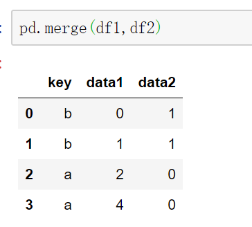
>>>print(pd.merge(d1,d2))#The default parameter how is the inner connection and will be merged according to the same field key, which is equivalent to on = 'key'.
key data1 data2
0 a 0 3
1 b 1 4
2 c 2 5
3 d 3 6That is, when merging two tables, if you do not add any other parameter descriptions, it defaults to inner. That is, there will be results only if the keyword keys have something in common (it can be understood as intersection. For example, keys in d1 and d2 have a, B, C and D, while d2 has no e and F, so there are only a, B, C and D in the consolidated table). Of course, duplicate items in the key column of the table are also allowed. They will not be deleted and changed during consolidation, as shown in the figure below.
When the merged fields on both sides are different, you can use left_on and right_ The on parameter sets the merge field. Of course, the merge fields here are all keys, so left_on and right_ The on parameter values are all keys.
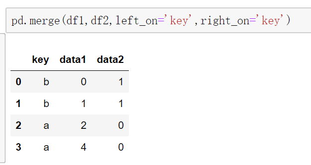
Some friends will be curious. What will happen if you don't use key here?
>>>print(pd.merge(d1,d2,left_on='data1',right_on='data2'))
  key_x  data1 key_y  data2
0     d      3     a      3
1     e      4     b      4
2     f      5     c      5
Changing 'data2' to True here will have the same effect. I believe smart friends have guessed that the merged keyword column should meet a basic requirement without indicating how: it has the same value, otherwise it will report an error (this is the understanding of intersection, empty set certainly can't duck!)
By the way, the key above_ x and key_x and y of Y are suffixes generated because the keys in the two tables have the same name. Just like you create a text called "learning materials" on the computer desktop in your life, and then create a new text, also known as "learning materials", but after you name it and press enter, it will automatically change to "learning materials (1)". Similarly, the text can be renamed, and this place can also be renamed! (well, it is distinguished by adding a suffix)
>>>print(pd.merge(d1,d2,left_on='data1',right_index=True,suffixes=('A','B')))
  keyA  data1 keyB  data2
0    a      0    a      3
1    b      1    b      4
2    c      2    c      5
3    d      3    d      6
Since there is intersection, there must be union according to mathematical thinking. you 're right! That's outer!
The connection modes of merge mainly include inner connection, outer connection, left connection and right connection. When outer connection is adopted, union will be taken and filled with NaN.
>>>print(pd.merge(d1,d2,how='outer',left_on='data1',right_index=True,suffixes=('A','B')))
  keyA  data1 keyB  data2
0    a      0    a    3.0
1    b      1    b    4.0
2    c      2    c    5.0
3    d      3    d    6.0
4    e      4  NaN    NaN
5    f      5  NaN    NaN
(2)append
result = df1.append(df2)

Here I also have a link to access the information. Please help yourself.
The append method of DataFrame of pandas is introduced in detail
There are many formats that can be added to append, one of which is a dictionary
>>>import pandas as pd
>>>d1=pd.DataFrame({'key':list('abcdef'),'data1':range(6)})
>>>data=pd.DataFrame()
>>>print(data)
Empty DataFrame
Columns: []
Index: []

>>>a={"x":1,"y":2}
>>>data=data.append(a,ignore_index=True)
>>>print(data)
     x    y
0  1.0  2.0

>>>data=data.append(d1,ignore_index=True)
>>>print(data)
     x    y  key  data1
0  1.0  2.0  NaN    NaN
1  NaN  NaN    a    0.0
2  NaN  NaN    b    1.0
3  NaN  NaN    c    2.0
4  NaN  NaN    d    3.0
5  NaN  NaN    e    4.0
6  NaN  NaN    f    5.0
ignore_index=True when adding a dictionary, otherwise an error will be reported. However, there are special cases in non dictionary cases (that is, the same index will appear when using append multiple times, and then an error will be reported). It is recommended to form a habit and type this code to save your life.
Add the list directly. There's no big problem. You may need to pay attention to the dimension of the list: one-dimensional columns, two-dimensional rows, and three-dimensional lists are empty.
>>>data = pd.DataFrame()
>>>a = [[[1,2,3]]]
>>>data = data.append(a)
>>>print(data)
           0
0  [1, 2, 3]
(3)join
After consulting some materials, konjaku found that it was OK to master merge. join and merge are very similar. I won't go into too much detail here. The big guy links, and everyone is free (in fact, I can't write, and it's easy for everyone to understand)
(4)concat
Careful friends also found that this is another article written by the big man of merge, which is convenient for understanding as a reference.
[Python3]pandas. Detailed explanation of concat usage
2. Set index column
df_inner=df_inner.set_index('id')
#Help you recall these two data sheets
>>>df1=pd.DataFrame({"id":[1001,1002,1003,1004,1005,1006,1007,1008],
"gender":['male','female','male','female','male','female','male','female'],
"pay":['Y','N','Y','Y','N','Y','N','Y',],
"m-point":[10,12,20,40,40,40,30,20]})
>>>print(df1)
     id  gender pay  m-point
0  1001    male   Y       10
1  1002  female   N       12
2  1003    male   Y       20
3  1004  female   Y       40
4  1005    male   N       40
5  1006  female   Y       40
6  1007    male   N       30
7  1008  female   Y       20

>>>print(df)
     id       date         city category  age   price
0  1001 2013-01-02     Beijing     100-A   23  1200.0
1  1002 2013-01-03           SH    100-B   44     NaN
2  1003 2013-01-04   guangzhou     110-A   54  2133.0
3  1004 2013-01-05     Shenzhen    110-C   32  5433.0
4  1005 2013-01-06     shanghai    210-A   34     NaN
5  1006 2013-01-07     BEIJING     130-F   32  4432.0

>>>df_inner=pd.merge(df,df1,how='inner')  # Match, merge, intersection
>>>print(df_inner)
     id       date         city category  age   price  gender pay  m-point
0  1001 2013-01-02     Beijing     100-A   23  1200.0    male   Y       10
1  1002 2013-01-03           SH    100-B   44     NaN  female   N       12
2  1003 2013-01-04   guangzhou     110-A   54  2133.0    male   Y       20
3  1004 2013-01-05     Shenzhen    110-C   32  5433.0  female   Y       40
4  1005 2013-01-06     shanghai    210-A   34     NaN    male   N       40
5  1006 2013-01-07     BEIJING     130-F   32  4432.0  female   Y       40

>>>df_inner=df_inner.set_index('id')
>>>print(df_inner)
           date         city category  age   price  gender pay  m-point
id
1001 2013-01-02     Beijing     100-A   23  1200.0    male   Y       10
1002 2013-01-03           SH    100-B   44     NaN  female   N       12
1003 2013-01-04   guangzhou     110-A   54  2133.0    male   Y       20
1004 2013-01-05     Shenzhen    110-C   32  5433.0  female   Y       40
1005 2013-01-06     shanghai    210-A   34     NaN    male   N       40
1006 2013-01-07     BEIJING     130-F   32  4432.0  female   Y       40
3. Sort by the value of a specific column
df_inner.sort_values(by=['age'])
>>>print(df_inner.sort_values(by=['age']))
     id       date         city category  age   price  gender pay  m-point
0  1001 2013-01-02     Beijing     100-A   23  1200.0    male   Y       10
3  1004 2013-01-05     Shenzhen    110-C   32  5433.0  female   Y       40
5  1006 2013-01-07     BEIJING     130-F   32  4432.0  female   Y       40
4  1005 2013-01-06     shanghai    210-A   34     NaN    male   N       40
1  1002 2013-01-03           SH    100-B   44     NaN  female   N       12
2  1003 2013-01-04   guangzhou     110-A   54  2133.0    male   Y       20
4. Sort by index column
df_inner.sort_index()
>>>df_inner=df_inner.set_index('age')
>>>print(df_inner)
       id       date         city category   price  gender pay  m-point
age
23   1001 2013-01-02     Beijing     100-A  1200.0    male   Y       10
44   1002 2013-01-03           SH    100-B     NaN  female   N       12
54   1003 2013-01-04   guangzhou     110-A  2133.0    male   Y       20
32   1004 2013-01-05     Shenzhen    110-C  5433.0  female   Y       40
34   1005 2013-01-06     shanghai    210-A     NaN    male   N       40
32   1006 2013-01-07     BEIJING     130-F  4432.0  female   Y       40

>>>print(df_inner.sort_index())
       id       date         city category   price  gender pay  m-point
age
23   1001 2013-01-02     Beijing     100-A  1200.0    male   Y       10
32   1004 2013-01-05     Shenzhen    110-C  5433.0  female   Y       40
32   1006 2013-01-07     BEIJING     130-F  4432.0  female   Y       40
34   1005 2013-01-06     shanghai    210-A     NaN    male   N       40
44   1002 2013-01-03           SH    100-B     NaN  female   N       12
54   1003 2013-01-04   guangzhou     110-A  2133.0    male   Y       20
5. If the value in the price column is > 3000, the group column displays high, otherwise it displays low
Here we will talk about a little knowledge of numpy. The role of where is whether the conditions are met. If it is met, it returns the result of the previous option, and if not, it returns the latter. (group is created without)
df_inner['group'] = np.where(df_inner['price'] > 3000,'high','low')
>>>df_inner['group'] = np.where(df_inner['price'] > 3000,'high','low')
>>>print(df_inner)
     id       date         city category  ...  gender  pay m-point group
0  1001 2013-01-02     Beijing     100-A  ...    male    Y      10   low
1  1002 2013-01-03           SH    100-B  ...  female    N      12   low
2  1003 2013-01-04   guangzhou     110-A  ...    male    Y      20   low
3  1004 2013-01-05     Shenzhen    110-C  ...  female    Y      40  high
4  1005 2013-01-06     shanghai    210-A  ...    male    N      40   low
5  1006 2013-01-07     BEIJING     130-F  ...  female    Y      40  high

[6 rows x 10 columns]
6. Group and mark the data with multiple conditions
df_inner.loc[(df_inner['city'] == 'beijing') & (df_inner['price'] >= 4000), 'sign']=1
>>>df_inner.loc[(df_inner['city'] == 'beijing') | (df_inner['price'] >= 4000), 'sign']=1
>>>print(df_inner)
     id       date         city category  ...  gender  pay m-point sign
0  1001 2013-01-02     Beijing     100-A  ...    male    Y      10  NaN
1  1002 2013-01-03           SH    100-B  ...  female    N      12  NaN
2  1003 2013-01-04   guangzhou     110-A  ...    male    Y      20  NaN
3  1004 2013-01-05     Shenzhen    110-C  ...  female    Y      40  1.0
4  1005 2013-01-06     shanghai    210-A  ...    male    N      40  NaN
5  1006 2013-01-07     BEIJING     130-F  ...  female    Y      40  1.0

[6 rows x 10 columns]
After learning this, you guys actually have a feeling about the routine, so I won't repeat it and carry it directly!
7. List the values of the category field in turn, and create a data table. The index value is DF_ The index column of inner is called category and size
pd.DataFrame((x.split('-') for x in df_inner['category']),index=df_inner.index,columns=['category','size']))
8. The split data sheet and the original DF will be completed_ Match the inner data table
df_inner=pd.merge(df_inner,split,right_index=True, left_index=True)
6, Data extraction
Three main functions are used: loc,iloc and ix. loc function extracts by tag value, iloc extracts by location, and ix can extract by tag and location at the same time.
1. Extract the value of a single line by index
You can extract a row by changing the value in parentheses.
df_inner.loc[3]
>>>print(df_inner.loc[3])
id                         1004
date        2013-01-05 00:00:00
city                   Shenzhen
category                  110-C
age                          32
price                      5433
gender                   female
pay                           Y
m-point                      40
Name: 3, dtype: object
#Note that this is a row, but it is represented as a column
2. Extract area row values by index
By changing the scope.
df_inner.iloc[0:5]
>>>print(df_inner.iloc[0:4])
     id       date         city category  age   price  gender pay  m-point
0  1001 2013-01-02     Beijing     100-A   23  1200.0    male   Y       10
1  1002 2013-01-03           SH    100-B   44     NaN  female   N       12
2  1003 2013-01-04   guangzhou     110-A   54  2133.0    male   Y       20
3  1004 2013-01-05     Shenzhen    110-C   32  5433.0  female   Y       40
3. Reset Index & set other indexes & extract selected index data
Some operations are to set index columns, while resetting is the reverse operation.
Attention! For extracting the selected data, if the index is in str format, the method of ['strA':'strB'] is adopted. If it is in int format, it must be extracted in the normal order!
df_inner=df_inner.set_index('age')
df_inner.reset_index()
df_inner=df_inner.set_index('date')
df_inner[:'2013-01-04']
>>>print(df_inner)
     id       date         city category  age   price  gender pay  m-point
0  1001 2013-01-02     Beijing     100-A   23  1200.0    male   Y       10
1  1002 2013-01-03           SH    100-B   44     NaN  female   N       12
2  1003 2013-01-04   guangzhou     110-A   54  2133.0    male   Y       20
3  1004 2013-01-05     Shenzhen    110-C   32  5433.0  female   Y       40
4  1005 2013-01-06     shanghai    210-A   34     NaN    male   N       40
5  1006 2013-01-07     BEIJING     130-F   32  4432.0  female   Y       40

>>>df_inner=df_inner.set_index('age')
>>>print(df_inner)
       id       date         city category   price  gender pay  m-point
age
23   1001 2013-01-02     Beijing     100-A  1200.0    male   Y       10
44   1002 2013-01-03           SH    100-B     NaN  female   N       12
54   1003 2013-01-04   guangzhou     110-A  2133.0    male   Y       20
32   1004 2013-01-05     Shenzhen    110-C  5433.0  female   Y       40
34   1005 2013-01-06     shanghai    210-A     NaN    male   N       40
32   1006 2013-01-07     BEIJING     130-F  4432.0  female   Y       40

>>>print(df_inner[:'54'])
#report errors
>>>print(df_inner[:3])#First three digits of output
       id       date         city category   price  gender pay  m-point
age
23   1001 2013-01-02     Beijing     100-A  1200.0    male   Y       10
44   1002 2013-01-03           SH    100-B     NaN  female   N       12
54   1003 2013-01-04   guangzhou     110-A  2133.0    male   Y       20


>>>print(df_inner.reset_index())#Reset index
   age    id       date         city category   price  gender pay  m-point
0   23  1001 2013-01-02     Beijing     100-A  1200.0    male   Y       10
1   44  1002 2013-01-03           SH    100-B     NaN  female   N       12
2   54  1003 2013-01-04   guangzhou     110-A  2133.0    male   Y       20
3   32  1004 2013-01-05     Shenzhen    110-C  5433.0  female   Y       40
4   34  1005 2013-01-06     shanghai    210-A     NaN    male   N       40
5   32  1006 2013-01-07     BEIJING     130-F  4432.0  female   Y       40

>>>df_inner=df_inner.set_index('category')
>>>print(df_inner)
            id       date         city   price  gender pay  m-point
category
100-A     1001 2013-01-02     Beijing   1200.0    male   Y       10
100-B     1002 2013-01-03           SH     NaN  female   N       12
110-A     1003 2013-01-04   guangzhou   2133.0    male   Y       20
110-C     1004 2013-01-05     Shenzhen  5433.0  female   Y       40
210-A     1005 2013-01-06     shanghai     NaN    male   N       40
130-F     1006 2013-01-07     BEIJING   4432.0  female   Y       40

>>>print(df_inner[:'110-C'])
            id       date         city   price  gender pay  m-point
category
100-A     1001 2013-01-02     Beijing   1200.0    male   Y       10
100-B     1002 2013-01-03           SH     NaN  female   N       12
110-A     1003 2013-01-04   guangzhou   2133.0    male   Y       20
110-C     1004 2013-01-05     Shenzhen  5433.0  female   Y       40

>>>df_inner=df_inner.set_index('date')
>>>print(df_inner[:'2013-01-04'])
              id         city category  age   price  gender pay  m-point
date
2013-01-02  1001     Beijing     100-A   23  1200.0    male   Y       10
2013-01-03  1002           SH    100-B   44     NaN  female   N       12
2013-01-04  1003   guangzhou     110-A   54  2133.0    male   Y       20
The following are easy to understand and can be carried for everyone to see ~
4. Use iloc to extract data by location area
df_inner.iloc[:3,:2] #The number before and after the colon is no longer the label name of the index, but the position of the data, starting from 0, the first three rows and the first two columns.
5. Adapt to iloc lifting data separately by location
df_inner.iloc[[0,2,5],[4,5]] #Extract rows 0, 2 and 5, columns 4 and 5
6. Use ix to extract data by index label and location
df_inner.ix[:'2013-01-03',:4] #Before January 3, 2013, the first four columns of data
7. Judge whether the value of city column is Beijing
df_inner['city'].isin(['beijing'])
8. Judge whether beijing and shanghai are included in the city column, and then extract the qualified data
df_inner.loc[df_inner['city'].isin(['beijing','shanghai'])]
9. Extract the first three characters and generate a data table
pd.DataFrame(category.str[:3])
7, Data filtering
Use the and, or and non conditions to filter the data, count and sum the data.
1. Use "and", "or" and "not" to filter
About these three logical judgments and symbols, konjaku, who has been learning python before, is really strange, but when Xiao konjaku has the experience of learning C language, he finds that these three are really friendly ~ ~ ~ so everyone is not surprised, just remember.
df_inner.loc[(df_inner['age'] > 25) & (df_inner['city'] == 'beijing'), ['id','city','age','category','gender']]
#"And" = >&

df_inner.loc[(df_inner['age'] > 25) | (df_inner['city'] == 'beijing'), ['id','city','age','category','gender']].sort(['age'])
#"Or" = >|

df_inner.loc[(df_inner['city'] != 'beijing'), ['id','city','age','category','gender']].sort(['id'])
#"Not" = >=
2. Count the filtered data by city column
df_inner.loc[(df_inner['city'] != 'beijing'), ['id','city','age','category','gender']].sort(['id']).city.count()
3. Use the query function to filter
df_inner.query('city == ["beijing", "shanghai"]')
>>>print(df_inner.query('city == ["beijing", "shanghai"]'))
     id       date      city category  age  price gender pay  m-point
4  1005 2013-01-06  shanghai    210-A   34    NaN   male   N       40
4. Sum the filtered results according to prince
df_inner.query('city == ["beijing", "shanghai"]').price.sum()
>>>print(df_inner.query('city == ["beijing", "shanghai"]').price.sum())
0.0
#Because it is null, the sum is 0
8, Data summary
The main functions are groupby and pivot_ table
1. Count and summarize all columns
df_inner.groupby('city').count()
I don't need to say more about the specific understanding. You can understand it by looking at the comparison below.
>>>print(df_inner.groupby('city').count())
             id  date  category  age  price  gender  pay  m-point
city
 guangzhou    1     1         1    1      1       1    1        1
BEIJING       1     1         1    1      1       1    1        1
Beijing       1     1         1    1      1       1    1        1
SH            1     1         1    1      0       1    1        1
Shenzhen      1     1         1    1      1       1    1        1
shanghai      1     1         1    1      0       1    1        1

>>>print(df_inner.groupby('age').count())
     id  date  city  category  price  gender  pay  m-point
age
23    1     1     1         1      1       1    1        1
32    2     2     2         2      2       2    2        2
34    1     1     1         1      0       1    1        1
44    1     1     1         1      0       1    1        1
54    1     1     1         1      1       1    1        1
2. Count the id field by age
df_inner.groupby('age')['id'].count()
>>>print(df_inner.groupby('age')['id'].count())
age
23    1
32    2
34    1
44    1
54    1
Name: id, dtype: int64
3. Summarize and count the two fields
df_inner.groupby(['city','age'])['id'].count()
>>>print(df_inner.groupby(['city','age'])['id'].count())
city         age
 guangzhou   54     1
BEIJING      32     1
Beijing      23     1
SH           44     1
Shenzhen     32     1
shanghai     34     1
Name: id, dtype: int64
4. Summarize the city field and calculate the total and average value of prince respectively
df_inner.groupby('city')['price'].agg([len,np.sum, np.mean])
>>>print(df_inner.groupby('city')['price'].agg([len,np.sum, np.mean]))
             len     sum    mean
city
 guangzhou   1.0  2133.0  2133.0
BEIJING      1.0  4432.0  4432.0
Beijing      1.0  1200.0  1200.0
SH           1.0     0.0     NaN
Shenzhen     1.0  5433.0  5433.0
shanghai     1.0     0.0     NaN
9, Data statistics
1. Simple data sampling (random)
df_inner.sample(n=3)
>>>print(df_inner.sample(n=3))
     id       date      city category  age   price  gender pay  m-point
5  1006 2013-01-07  BEIJING     130-F   32  4432.0  female   Y       40
3  1004 2013-01-05  Shenzhen    110-C   32  5433.0  female   Y       40
0  1001 2013-01-02  Beijing     100-A   23  1200.0    male   Y       10

>>>print(df_inner.sample(n=3))
     id       date      city category  age   price  gender pay  m-point
4  1005 2013-01-06  shanghai    210-A   34     NaN    male   N       40
1  1002 2013-01-03        SH    100-B   44     NaN  female   N       12
5  1006 2013-01-07  BEIJING     130-F   32  4432.0  female   Y       40
2. Manually set the sampling weight
weights = [0, 0, 0, 0, 0.5, 0.5]
df_inner.sample(n=2, weights=weights)
>>>weights = [0, 0, 0, 0, 0.5, 0.5]
>>>print(df_inner.sample(n=2, weights=weights))
     id       date      city category  age   price  gender pay  m-point
5  1006 2013-01-07  BEIJING     130-F   32  4432.0  female   Y       40
4  1005 2013-01-06  shanghai    210-A   34     NaN    male   N       40
3. Do not put it back after sampling
df_inner.sample(n=6, replace=False)
4. Put it back after sampling
df_inner.sample(n=6, replace=True)
Next is statistics
(Ben konjaku learned it, but it's too troublesome to turn to the textbook for explanation, so I won't say more.)
5. Descriptive statistics of data sheet
df_inner.describe().round(2).T #The round function sets the display decimal places, and T represents transpose
>>>print(df_inner.describe().round(2))
            id    age    price  m-point
count     6.00   6.00     4.00     6.00
mean   1003.50  36.50  3299.50    27.00
std       1.87  10.88  1966.64    14.63
min    1001.00  23.00  1200.00    10.00
25%    1002.25  32.00  1899.75    14.00
50%    1003.50  33.00  3282.50    30.00
75%    1004.75  41.50  4682.25    40.00
max    1006.00  54.00  5433.00    40.00

>>>print(df_inner.describe().round(2).T) #The round function sets the display decimal places, and T represents transpose
         count    mean      std     min      25%     50%      75%     max
id         6.0  1003.5     1.87  1001.0  1002.25  1003.5  1004.75  1006.0
age        6.0    36.5    10.88    23.0    32.00    33.0    41.50    54.0
price      4.0  3299.5  1966.64  1200.0  1899.75  3282.5  4682.25  5433.0
m-point    6.0    27.0    14.63    10.0    14.00    30.0    40.00    40.0
6. Calculate the standard deviation of the column
df_inner['price'].std()
7. Calculate the covariance between the two fields
df_inner['price'].cov(df_inner['m-point'])
8. Covariance between all fields in the data table
df_inner.cov()
>>>print(df_inner.cov())
                  id          age         price       m-point
id          3.500000    -0.700000  3.243333e+03     25.400000
age        -0.700000   118.300000 -2.255833e+03    -31.000000
price    3243.333333 -2255.833333  3.867667e+06  28771.666667
m-point    25.400000   -31.000000  2.877167e+04    214.000000
9. Correlation analysis of two fields
df_inner['price'].corr(df_inner['m-point']) #The correlation coefficient is between - 1 and 1, close to 1 is positive correlation, close to - 1 is negative correlation, and 0 is uncorrelated
10. Correlation analysis of data sheet
df_inner.corr()
10, Data output
Can you understand everything below~
1. Write to Excel
df_inner.to_excel('excel_to_python.xlsx', sheet_name='bluewhale_cc')
2. Write to CSV
df_inner.to_csv('excel_to_python.csv')
11, Last words
Finally, thank you for seeing here. This article is over. The following is a screenshot of konjaku's reprint authorization and code summary, hey hey~

# -*- coding: utf-8 -*-
"""
Created on Tue Jul 20 16:27:43 2021

@author: 86133
"""
import numpy as np
import pandas as pd
df = pd.DataFrame({"id":[1001,1002,1003,1004,1005,1006],
                   "date":pd.date_range('20130102', periods=6),
                   "city":['Beijing ', 'SH', ' guangzhou ', 'Shenzhen', 'shanghai', 'BEIJING '],
                   "age":[23,44,54,32,34,32],
                   "category":['100-A','100-B','110-A','110-C','210-A','130-F'],
                   "price":[1200,np.nan,2133,5433,np.nan,4432]},
                   columns =['id','date','city','category','age','price'])
#print(df)
'''
print(df.shape)#Represents a dimension. For example, (6,6) represents a 6 * 6 table

print(df.info())#Basic information of data table (dimension, column name, data format, occupied space, etc.)

print(df.dtypes)#Format of each column of data


print(df["city"].dtypes)#A column format

print(df.isnull())#View null values for the entire table

print(df["price"].isnull())#View the null value of a column

print(df['age'])
print(df['age'].unique())#View unique values for a column

print(df.values)#View the values of the data table

print(df.columns)#View column names

print(df.head())#View the first 5 rows of data (if there are no numbers in parentheses, the default is 5)
print(df.tail())#View the last 5 rows of data (if there is no number in parentheses, it defaults to 5)

df=df.fillna('Null value')
print(df['price'])#Fill empty values with the number 0

print(df['price'])
print(df['price'].fillna(df['price'].mean()))
#Fill NA with the mean value of column prince (mean value: the sum of N-term values that are not null, divided by N. The total number of values > n)

print(df['city'])
df['city']=df['city'].map(str.strip)#Remove spaces and align. Clear the character space of the city field
print(df['city'])

print(df['city'])
df['city']=df['city'].str.upper()#Case conversion, upper to all uppercase, lower to all lowercase
print(df['city'])

df=df.fillna(0)
print(df['price'])
print(df['price'].astype('int'))#Change the data format to float


print(df.rename(columns={'category': 'category-size'}))#Change column name

df['city']=df['city'].map(str.strip).str.lower()
print(df['city'])
print(df['city'].drop_duplicates())#Duplicate values after deletion
print(df['city'].drop_duplicates(keep='last'))#Delete the first duplicate value

df['city']=df['city'].map(str.strip).str.lower()
print(df['city'].replace('sh', 'shanghai'))#Data replacement
'''


df1=pd.DataFrame({"id":[1001,1002,1003,1004,1005,1006,1007,1008],
"gender":['male','female','male','female','male','female','male','female'],
"pay":['Y','N','Y','Y','N','Y','N','Y',],
"m-point":[10,12,20,40,40,40,30,20]})
#print(df1)

#print(df)

df_inner=pd.merge(df,df1,how='inner')  # Match, merge, intersection
df_left=pd.merge(df,df1,how='left')        #
df_right=pd.merge(df,df1,how='right')
df_outer=pd.merge(df,df1,how='outer')  #Union
#print(df_inner)


'''
result = df1.append(df2)#Add up and down
result = left.join(right, on='key')#Add left and right
'''
'''
d1=pd.DataFrame({'key':list('abcdef'),'data1':range(6)})
#print(d1)
d2=pd.DataFrame({'key':['a','b','c','d'],'data2':range(3,7)})
#print(d2)
#print(pd.merge(d1,d2))
#print(pd.merge(d1,d2,left_on='data1',right_on='data2'))
print(pd.merge(d1,d2,how='outer',left_on='data1',right_index=True,suffixes=('A','B')))
'''
'''
d1=pd.DataFrame({'key':list('abcdef'),'data1':range(6)})
data=pd.DataFrame()
print(data)
a={"x":1,"y":2}
data=data.append(a,ignore_index=True)
print(data)
data=data.append(d1,ignore_index=True)
print(data)
'''

'''
df_inner=df_inner.set_index('id')
print(df_inner)

print(df_inner.sort_values(by=['age']))

df_inner=df_inner.set_index('age')
print(df_inner)
print(df_inner.sort_index())

df_inner['group'] = np.where(df_inner['price'] > 3000,'high','low')
print(df_inner)

df_inner.loc[(df_inner['city'] == 'beijing') | (df_inner['price'] >= 4000), 'sign']=1
print(df_inner)

print(pd.DataFrame((x.split('-') for x in df_inner['category']),index=df_inner.index,columns=['category','size']))

print(df_inner)
split=pd.DataFrame((x.split('-') for x in df_inner['category']),index=df_inner.index,columns=['category_0','size'])
df_inner=pd.merge(df_inner,split,right_index=True, left_index=True)
print(df_inner)

print(df_inner.loc[3])

print(df_inner.iloc[0:4])

print(df_inner)
df_inner=df_inner.set_index('age')
print(df_inner[:3])
df_inner=df_inner.set_index('category')
print(df_inner)
#print(df_inner.reset_index())#Reset index
print(df_inner[:'110-C'])

df_inner=df_inner.set_index('date')
print(df_inner)
print(df_inner[:'2013-01-04'])

print(df_inner['city'].isin(['shanghai']))

print(df_inner.loc[df_inner['city'].isin(['Beijing ','shanghai'])])

print(df_inner.loc[(df_inner['city'] != 'beijing'), ['id','city','age','category','gender']].sort(['id']).city.count())

print(df_inner.query('city == ["beijing", "shanghai"]'))

print(df_inner.query('city == ["beijing", "shanghai"]').price.sum())

print(df_inner.groupby('age').count())

print(df_inner.groupby('age')['id'].count())

print(df_inner.groupby(['city','age'])['id'].count())

print(df_inner.groupby('city')['price'].agg([len,np.sum, np.mean]))

print(df_inner.sample(n=3))

weights = [0, 0, 0, 0, 0.5, 0.5]
print(df_inner.sample(n=2, weights=weights))

print(df_inner)
print(df_inner.sample(n=3, replace=False))
print(df_inner)

print(df_inner.sample(n=3, replace=True))
print(df_inner)

print(df_inner.describe().round(2).T) #The round function sets the display decimal places, and T represents transpose
'''
print(df_inner.cov())