Poisson Distribution

Posted by mitchell on Fri, 11 Feb 2022 09:40:56 +0100

definition:

Real life is mostly subject to Poisson distribution

Suppose you work in a call center, how many calls will you receive in a day? It can be any number. Now, the total number of calls in a call center in a day can be modeled by Poisson distribution. Here are some examples:

The number of emergency calls recorded by the hospital in a day.
The number of thefts reported in a given area in one day.
Number of clients arriving at the salon within one hour.
The number of typographical errors per page in the book. Poisson distribution is suitable for events in random time and space, in which we only focus on the number of events.

When the following assumptions are valid, they are called Poisson distribution

Any successful event should not affect another successful event.
The probability of success in a short time must be equal to the probability of success in a longer time.
When the time interval is very small, the probability of success tends to zero within a given interval.

These symbols are used in Poisson distribution:

λ Is the rate at which events occur
t is the length of the time interval
X is the number of events in the interval.
Among them, X is called Poisson random variable, and the probability distribution of X is called Poisson distribution.
order μ Represents the average number of events in an interval of length t. So, um= λ* t.

For example, in a hospital, the probability of each patient coming to see a doctor is random and independent, then the total number of patients admitted to the hospital in a day (or other specific time period, an hour, a week, etc.) can be regarded as a random variable subject to poisson distribution. But why can this be done? Popular definition: it is assumed that an event occurs randomly over a period of time and meets the following conditions:

(1) The time period is infinitely divided into several small time periods. In this small time period close to zero, the probability of the event occurring once is directly proportional to the length of this minimum time period.
(2) In each minimal time period, the probability of the event occurring twice or more is equal to zero.
(3) The occurrence of this event is independent of each other in different small time periods.

This event is called poisson process. This second definition is more convenient for you to understand. Back to the example of hospital, if we divide a day into 24 hours, or 24x60 minutes, or 24x3600 seconds. The shorter the time, the smaller the probability of patients coming during this time period (for example, is the probability of patients coming to the hospital between 12:00 noon and 12:00 noon close to zero?). Condition one meets. In addition, if we divide the time very carefully, is it impossible for two patients (or more than two patients) to come at the same time? Even if two patients come at the same time, there is always one person who steps into the hospital gate first. Condition 2 is also met. But the requirements of condition three are relatively harsh. When applied to practical examples, it means that the probability of patients coming to the hospital must be independent of each other. If not, it can not be regarded as poisson distribution.

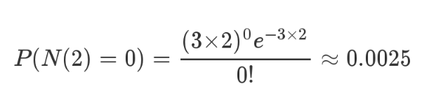
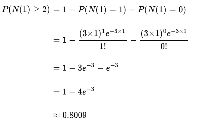
It is known that an average of three babies are born per hour. How many babies will be born in the next hour?

It's possible to be born six at a time, or it's possible not to be born at all. This is something we can't know.

Poisson distribution is to describe the specific occurrence probability of an event in a certain period of time.

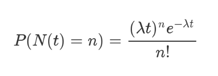
The above is the formula of Poisson distribution. To the left of the equal sign, P stands for probability, n stands for some functional relationship, t stands for time, n stands for quantity, and the probability of three babies born within one hour is expressed as P(N(1) = 3). To the right of the equal sign, λ Indicates the frequency of the event.

For the next two hours, the probability that a baby will not be born is 0.25%, which is basically impossible.

The probability of having at least two babies in the next hour is 80%.

# IMPORTS
import numpy as np
import scipy.stats as stats
import matplotlib.pyplot as plt
import matplotlib.style as style
from IPython.core.display import HTML

# PLOTTING CONFIG
%matplotlib inline
style.use('fivethirtyeight')
plt.rcParams["figure.figsize"] = (14, 7)

plt.figure(dpi=100)

# PDF
plt.bar(x=np.arange(20), 
        height=(stats.poisson.pmf(np.arange(20), mu=5)), 
        width=.75,
        alpha=0.75
       )

# CDF
plt.plot(np.arange(20), 
         stats.poisson.cdf(np.arange(20), mu=5),
         color="#fc4f30",
        )

# LEGEND
plt.text(x=8, y=.45, s="pmf (normed)", alpha=.75, weight="bold", color="#008fd5")
plt.text(x=8.5, y=.9, s="cdf", alpha=.75, weight="bold", color="#fc4f30")

# TICKS
plt.xticks(range(21)[::2])
plt.tick_params(axis = 'both', which = 'major', labelsize = 18)
plt.axhline(y = 0.005, color = 'black', linewidth = 1.3, alpha = .7)

# TITLE, SUBTITLE & FOOTER
plt.text(x = -2.5, y = 1.25, s = "Poisson Distribution - Overview",
               fontsize = 26, weight = 'bold', alpha = .75)
plt.text(x = -2.5, y = 1.1, 
         s = 'Depicted below are the normed probability mass function (pmf) and the cumulative density\nfunction (cdf) of a Poisson distributed random variable $ y \sim Poi(\lambda) $, given $ \lambda = 5 $.',
         fontsize = 19, alpha = .85)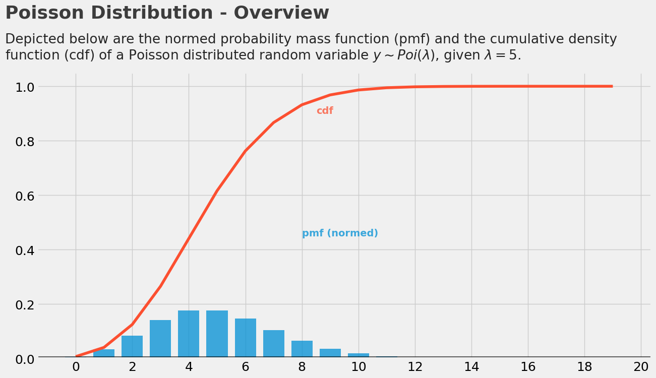

Change parameters λ:

plt.figure(dpi=100)

# PDF LAM = 1
plt.scatter(np.arange(20),
            (stats.poisson.pmf(np.arange(20), mu=1)),#/np.max(stats.poisson.pmf(np.arange(20), mu=1))),
            alpha=0.75,
            s=100
       )
plt.plot(np.arange(20),
         (stats.poisson.pmf(np.arange(20), mu=1)),#/np.max(stats.poisson.pmf(np.arange(20), mu=1))),
         alpha=0.75,
        )

# PDF LAM = 5
plt.scatter(np.arange(20),
            (stats.poisson.pmf(np.arange(20), mu=5)),
            alpha=0.75,
            s=100
       )
plt.plot(np.arange(20),
         (stats.poisson.pmf(np.arange(20), mu=5)),
         alpha=0.75,
        )

# PDF LAM = 10
plt.scatter(np.arange(20),
            (stats.poisson.pmf(np.arange(20), mu=10)),
            alpha=0.75,
            s=100
       )
plt.plot(np.arange(20),
         (stats.poisson.pmf(np.arange(20), mu=10)),
         alpha=0.75,
        )

# LEGEND
plt.text(x=3, y=.1, s="$\lambda = 1$", alpha=.75, rotation=-65, weight="bold", color="#008fd5")
plt.text(x=8.25, y=.075, s="$\lambda = 5$", alpha=.75, rotation=-35, weight="bold", color="#fc4f30")
plt.text(x=14.5, y=.06, s="$\lambda = 10$", alpha=.75, rotation=-20, weight="bold", color="#e5ae38")

# TICKS
plt.xticks(range(21)[::2])
plt.tick_params(axis = 'both', which = 'major', labelsize = 18)
plt.axhline(y = 0, color = 'black', linewidth = 1.3, alpha = .7)

# TITLE, SUBTITLE & FOOTER
plt.text(x = -2.5, y = .475, s = "Poisson Distribution - $\lambda$",
               fontsize = 26, weight = 'bold', alpha = .75)
plt.text(x = -2.5, y = .425, 
         s = 'Depicted below are three Poisson distributed random variables with varying $\lambda $. As one can easily\nsee the parameter $\lambda$ shifts and flattens the distribution (the smaller $ \lambda $ the sharper the function).',
         fontsize = 19, alpha = .85)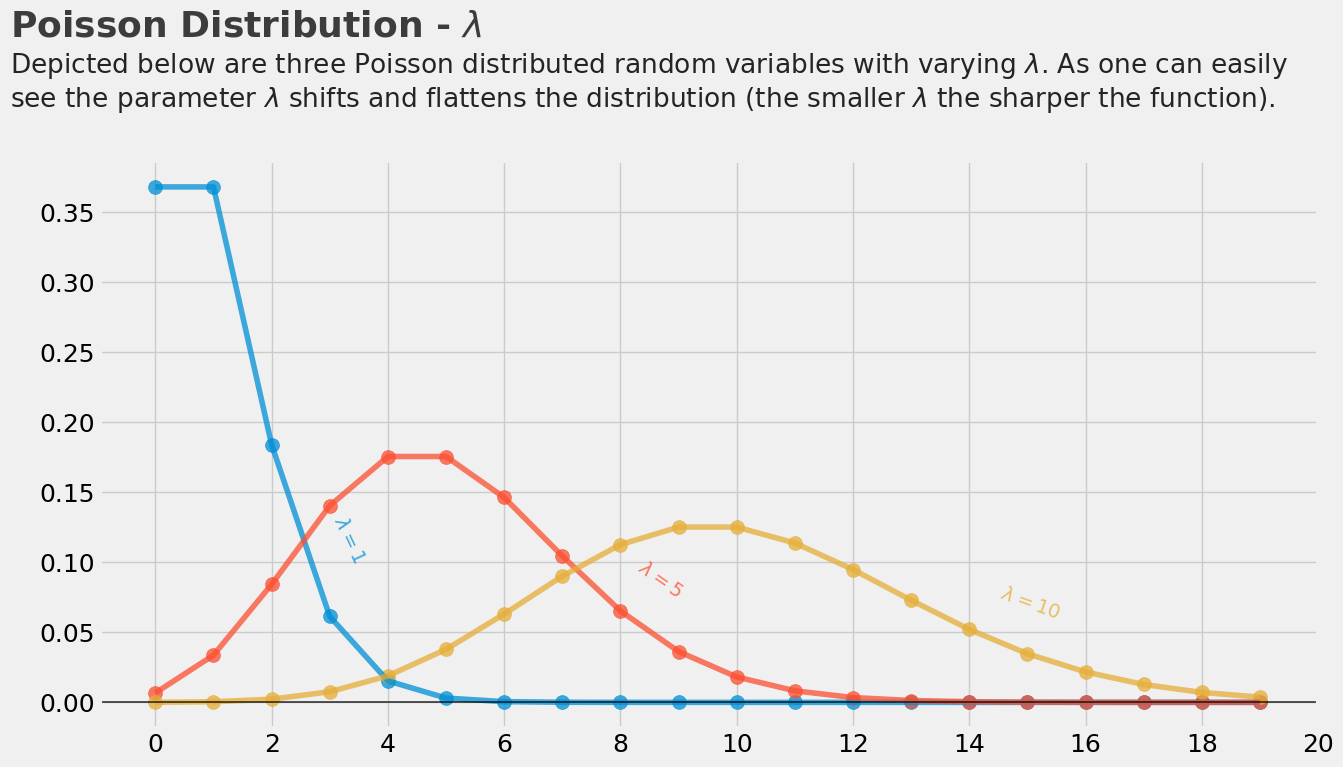

Construct random distribution:

import numpy as np
from scipy.stats import poisson

# draw a single sample
np.random.seed(42)
print(poisson.rvs(mu=10), end="\n\n")

# draw 10 samples
print(poisson.rvs(mu=10, size=10), end="\n\n")

12

[ 6 11 14  7  8  9 11  8 10  7]

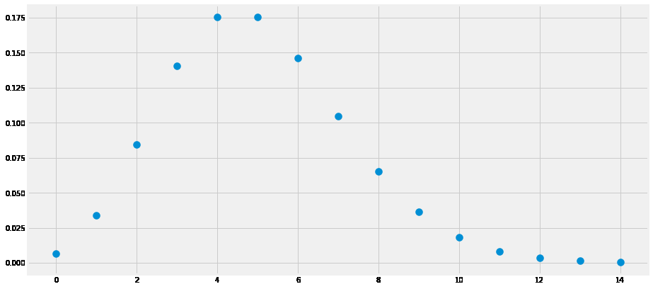
Draw the probability density function:

from scipy.stats import poisson

# additional imports for plotting purpose
import numpy as np
import matplotlib.pyplot as plt
%matplotlib inline
plt.rcParams["figure.figsize"] = (14,7)


# continuous pdf for the plot
x_s = np.arange(15)
y_s = poisson.pmf(k=x_s, mu=5)
plt.scatter(x_s, y_s, s=100);

Calculate the probability of cumulative probability density function:

from scipy.stats import poisson

# probability of x less or equal 0.3
print("P(X <=3) = {}".format(poisson.cdf(k=3, mu=5)))

# probability of x in [-0.2, +0.2]
print("P(2 < X <= 8) = {}".format(poisson.cdf(k=8, mu=5) - poisson.cdf(k=2, mu=5)))

P(X <=3) = 0.2650259152973616
P(2 < X <= 8) = 0.8072543457950705

Draw λ:

from collections import Counter

plt.figure(dpi=100)

##### COMPUTATION #####
# DECLARING THE "TRUE" PARAMETERS UNDERLYING THE SAMPLE
lambda_real = 7

# DRAW A SAMPLE OF N=1000
np.random.seed(42)
sample = poisson.rvs(mu=lambda_real, size=1000)

# ESTIMATE MU AND SIGMA
lambda_est = np.mean(sample)
print("Estimated LAMBDA: {}".format(lambda_est))

##### PLOTTING #####
# SAMPLE DISTRIBUTION
cnt = Counter(sample)
_, values = zip(*sorted(cnt.items()))
plt.bar(range(len(values)), values/np.sum(values), alpha=0.25);

# TRUE CURVE
plt.plot(range(18), poisson.pmf(k=range(18), mu=lambda_real), color="#fc4f30")

# ESTIMATED CURVE
plt.plot(range(18), poisson.pmf(k=range(18), mu=lambda_est), color="#e5ae38")

# LEGEND
plt.text(x=6, y=.06, s="sample", alpha=.75, weight="bold", color="#008fd5")
plt.text(x=3.5, y=.14, s="true distrubtion", rotation=60, alpha=.75, weight="bold", color="#fc4f30")
plt.text(x=1, y=.08, s="estimated distribution", rotation=60, alpha=.75, weight="bold", color="#e5ae38")

# TICKS
plt.xticks(range(17)[::2])
plt.tick_params(axis = 'both', which = 'major', labelsize = 18)
plt.axhline(y = 0.0009, color = 'black', linewidth = 1.3, alpha = .7)

# TITLE, SUBTITLE & FOOTER
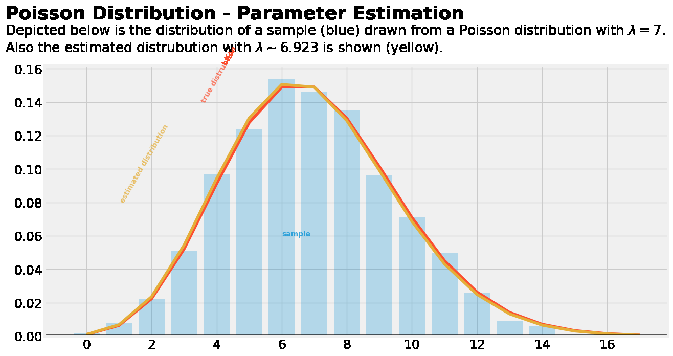
plt.text(x = -2.5, y = 0.19, s = "Poisson Distribution - Parameter Estimation",
               fontsize = 26, weight = 'bold', alpha = .75)
plt.text(x = -2.5, y = 0.17, 
         s = 'Depicted below is the distribution of a sample (blue) drawn from a Poisson distribution with $\lambda = 7$.\nAlso the estimated distrubution with $\lambda \sim {:.3f}$ is shown (yellow).'.format(np.mean(sample)),
         fontsize = 19, alpha = .85)

Topics: Python

Programmer Think

Poisson Distribution

definition:

Hot Topics