Poisson and Poisson like regression models are often used in count based data sets, that is, data containing integer counts. For example, the number of people entering the hospital emergency room per hour is such a data set.

Linear or nonlinear models based on ordinary least squares regression (such as linear models based on neural network regression technology) are not suitable for such data sets because they can predict negative values.

If the data set is a counted time series, there will be additional modeling complexity because the time series data is usually autocorrelated. Previous counts affect the value of future counts. If the regression model cannot fully capture the "information" contained in these correlations, "unexplained" information will leak into the residual of the model in the form of autocorrelation error. In this case, the goodness of fit of the model will be very poor.

The general remedies for this problem are as follows:

1. Before fitting the regression model, check whether the time series is seasonal, and if so, make seasonal adjustment. This makes sense even if there is seasonal autocorrelation.
2. The first difference of time series is made for all t, i.e. y_t - y_(t-1), and carry out white noise test on the differential time series. If the difference time series is white noise, the original time series is random walk. In this case, no further modeling is required.
3. Fit the regression model based on Poisson (or correlation) count on the seasonally adjusted time series, but include the lagged copy of the dependent variable y as the regression variable.

In this paper, we will explain how to use method (3) to fit Poisson or quasi Poisson models on the counted time series.

Manufacturing strings dataset

To illustrate the model fitting process, we will use the following open source data sets widely used in regression modeling Literature:

The data is a monthly time series showing the relationship between us manufacturing activity (off trend) and the number of US manufacturing contract strikes from 1968 to 1976.

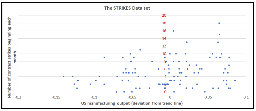
This data can be obtained using the statsmodels dataset package.

The dependent variable y is the number of strikes.

We'll start by importing all the necessary packages:

import statsmodels.api as sm
import statsmodels.discrete.discrete_model as dm
import numpy as np
from patsy import dmatrices
import statsmodels.graphics.tsaplots as tsa
from matplotlib import pyplot as plt

Let's use statsmodels to load the dataset into memory:

strikes_dataset = sm.datasets.get_rdataset(dataname='StrikeNb', package='Ecdat')

Print out dataset:

print(strikes_dataset.data)

We see the following output:

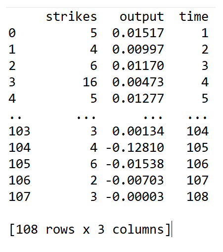
We regard the first 92 data points as training sets and the remaining 16 data points as test data sets

strikes_data = strikes_dataset.data.copy()
strikes_data_train = strikes_data.query('time<=92')
strikes_data_test = strikes_data.query('time>92').reset_index().drop('index', axis=1)

Print out the statistics of dependent variables:

print('Mean='+str(np.mean(strikes_data_train['strikes'])) + ' Variance='+str(np.var(strikes_data_train['strikes'])))

We get the following output:

Mean=5.5 Variance=14.728260869565217

We see that y is too scattered, so it violates the mean = variance assumption of Poisson model. In order to solve the problem of over dispersion, we will fit the negative binomial regression model with the following NB2 variance function:

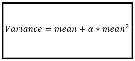
This is our regression expression. Strike is a dependent variable and output is our explanatory variable. Assuming regression intercept:

expr = 'strikes ~ output

We will use Patsy to calculate the X and y matrices. Patsy automatically adds a regression intercept column to X:

y_train, X_train = dmatrices(expr, strikes_data_train, return_type='dataframe')
print(y_train)
print(X_train)

y_test, X_test = dmatrices(expr, strikes_data_test, return_type='dataframe')
print(y_test)
print(X_test)

Construct and train the negative binomial regression model using NB2 variance function:

nb2_model = dm.NegativeBinomial(endog=y_train, exog=X_train, loglike_method='nb2')
nb2_model_results = nb2_model.fit(maxiter=100)
print(nb2_model_results.summary())

We get the following output of the fitted model summary:

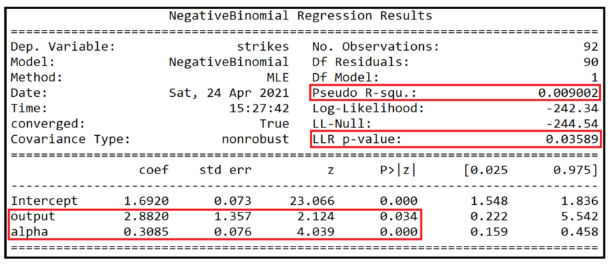
As shown by the p values of the coefficients (0.034 and 0.000), the output and dispersion parameters alpha are statistically significant at 95% confidence.

Fit degree

The pseudo R square is only 0.9%, indicating that the fitting quality of the training data set is very poor.

The p value of log likelihood ratio test is 0.03589, indicating that the model does better than intercept only model (also known as zero model) at 95% confidence level, but does not perform well at 99% or higher confidence level.

Let's take a look at the autocorrelation diagram of the residuals of the fitted model:

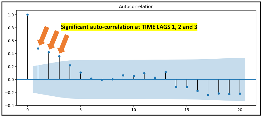
We can see that the residual error is autocorrelated when the time lag is 1, 2 and 3, which indicates that there is autocorrelation in the dependent variable strike, because the NB2 model can not fully explain the cause of leakage into the model residual.

Overall, the goodness of fit of this model is very poor.

Establish autoregressive Poisson model

In order to solve the case of residual autocorrelation, we will introduce the lagging copy of Y, specifically y_(t-1),y_(t-2) and y_(t-3) regression variables as output variables. But we don't introduce y directly_ (t-k) as a regression variable, but ln[y_(t-k)] is used to solve y_(t-k) the problem of "model explosion" when the coefficient is positive.

However, the use of ln() transformation raises a problem, that is, how to deal with the y of 0_ T is undefined for this logarithm. So we use the following techniques outlined by Cameron and Trivedi in their book Regression Analysis of Count Data (see section 7.5: autoregressive models) to solve this problem:

We will define a new index variable D for each delay of interest_ t. As follows:

• When y_ When t = 0: d_t=1, we will y_t is set to 0.
• When y_t > 0: d_ When t = 0, we will y_t keep it as it is.

Let's make these changes to the dataframe. Create a new column stripes_ Adj, set to 1 if stripes < 1, otherwise set to stripes:

strikes_data['strikes_adj'] = np.maximum(1, strikes_data['strikes'])

Define a function to set the indicator variable D_ The value of T, as described above.

def indicator_func(x):
    if x == 0:
        return 1
    else:
        return 0

And use this function to create a new indicator variable column:

strikes_data['d'] = strikes_data['strikes'].apply(indicator_func)

Now it's stripes_ Adj and d create lag variables:

strikes_data['ln_strikes_adj_lag1'] = strikes_data['strikes_adj'].shift(1)
strikes_data['ln_strikes_adj_lag2'] = strikes_data['strikes_adj'].shift(2)
strikes_data['ln_strikes_adj_lag3'] = strikes_data['strikes_adj'].shift(3)

strikes_data['d_lag1'] = strikes_data['d'].shift(1)
strikes_data['d_lag2'] = strikes_data['d'].shift(2)
strikes_data['d_lag3'] = strikes_data['d'].shift(3)

Delete all rows with empty cells:

strikes_data = strikes_data.dropna()

Finally, take a natural log ln_strikes_adj_lag1. Recall that we want to add the lag variable y_ (t_1)，y_ (t_2) and Y_ The natural logarithm of (t_3).

Let's see what our data looks like now:

print(strikes_data)

Let's divide the data into training and test data sets again:

strikes_data_train=strikes_data.query('time<=92')
strikes_data_test=strikes_data.query('time>92').reset_index().drop('index', axis=1)

Our regression expression also needs to be updated to include lag variables:

expr = 'strikes ~ output + ln_strikes_adj_lag1 + ln_strikes_adj_lag2 + ln_strikes_adj_lag3 + d_lag1 + d_lag2 + d_lag3'

Using Patsy, the y and X matrices can be obtained:

y_train, X_train = dmatrices(expr, strikes_data_train, return_type='dataframe')
print(y_train)
print(X_train)

Finally, we will build and fit the regression model on (y_train, X_train). This time, we will use the direct Poisson regression model:

poisson_model = dm.Poisson(endog=y_train, exog=X_train)
poisson_model_results = poisson_model.fit(maxiter=100)
print(poisson_model_results.summary()

We see the following results:

Fit degree

First of all, it should be noted that the goodness of fit measured by pseudor squared is 0.9% to 15.69% higher than that of the early NB2 model. This is a great progress. This time, the p value of LLR test is also very small, which is 1.295e-15. This means that we can say with close to 100% confidence that the Poisson model with lag variable is better than the intercept model. In retrospect, we can say that there is only 95% confidence.

Let's take a look at the autocorrelation diagram of the residuals of this lag variable Poisson model:

tsa.plot_acf(poisson_model_results.resid, alpha=0.05)
plt.show()

We see the following figure:

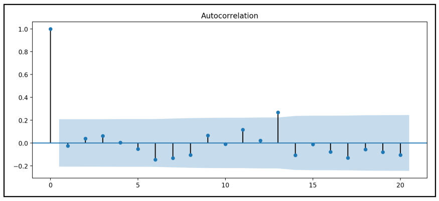
Except for the very slight significant correlation at LAG 13, the correlation between the residuals and all other lags is well within the specified alpha range.

Our strategy of adding lagged strike copies to the regression variables of Poisson model seems to have explained the autocorrelation in many strike variables.

Meaning of variables

We summarize the coefficients, output, LN of the Poisson model with lag variables from the training attention_ strikes_ adj_ Lag1 and ln_strikes_adj_lag2 is important at the 95% confidence level, the third lag ln_strikes_adj_lag3 is an important coefficient, and only about 75% confidence level indicates an assumed value of 0.237. In addition, three lag indicator variables d_lag1,d_lag2 and d_lag3 was not statistically significant at 95% confidence level.

forecast

Let's use the fitted lag variable Poisson model to predict the number of strikes in our previously reserved test data set. We should not hope that the quality of forecasts is too high. Remember that although this model fits much better than the previous NB2 model, the pseudo R-square is still only 16%.

We will use Patsy to view (y_test, X_test):

y_test, X_test = dmatrices(expr, strikes_data_test, return_type='dataframe')
print(y_test)
print(X_test)

To X_test to predict:

poisson_predictions = poisson_model_results.predict(X_test

Plot predicted and actual values:

predicted_counts=poisson_predictions
actual_counts = y_test['strikes']
fig = plt.figure()
fig.suptitle('Predicted versus actual strike counts')
predicted, = plt.plot(X_test.index, predicted_counts, 'go-', label='Predicted counts')
actual, = plt.plot(X_test.index, actual_counts, 'ro-', label='Actual counts')
plt.legend(handles=[predicted, actual])
plt.show()

We get the following figure:

next step

We can try to improve the goodness of fit of the lag variable model through the following modifications:

In addition to the output, the first three time lags of the output variables are also used as regression variables.

The delay values of output variables and strike variables are used as regression variables.

The negative binomial model (using NB1 or NB2 variance function) is used to replace the Poisson model, and the lag variables of the above types are used as regression variables.

Papers and related links

Cameron A. Colin, Trivedi Pravin K., Regression Analysis of Count Data, Econometric Society Monograph №30, Cambridge University Press, 1998. ISBN: 0521635675

McCullagh P., Nelder John A., Generalized Linear Models, 2nd Ed., CRC Press, 1989, ISBN 0412317605, 9780412317606

Kennan J., The duration of contract strikes in U.S. manufacturing, Journal of Econometrics, Volume 28, Issue 1, 1985, Pages 5–28, ISSN 0304–4076, https://doi.org/10.1016/0304-4076(85)90064-8. PDF download link

Cameron C. A., Trivedi P. K., Regression-based tests for overdispersion in the Poisson model, Journal of Econometrics, Volume 46, Issue 3, 1990, Pages 347–364, ISSN 0304–4076, https://doi.org/10.1016/0304-4076(90)90014-K.

Author: Sachin Date

Deep hub translation group