Polynomial Regression Learning Notes

Posted by davidp on Fri, 07 Jun 2019 22:56:27 +0200

Operating system: CentOS 7.3.1611_x64

python version: 2.7.5

sklearn version: 0.18.2

tensorflow version: 1.2.1

Definition and manifestation of polynomials

Polynomial is a basic concept in algebra. It is an algebraic expression obtained by finite addition and subtraction, multiplication and power multiplication of natural numbers by variables called indefinite elements and constants called coefficients.

Polynomials are divided into univariate polynomials and multivariate polynomials, in which:

A polynomial with only one indefinite element is called a univariate polynomial.

Polynomials with more than one indefinite element are called multivariate polynomials.

This paper deals with the related problems of unary polynomials.

Its general form is as follows (python grammatical expression):

y = a0 + a1 * x + a2 * (x**2) + ... + an * (x ** n) + e

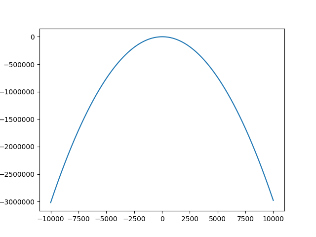
For example, the general quadratic polynomial regression model is as follows (python grammatical expression):

y = a0 + a1 * x + a2 * (x**2) + e

When a0,a1,a2,e = 10,2,-0.03,0.5, the general figure is as follows:

The source code is as follows:

#! /usr/bin/env python
#-*- coding:utf-8 -*-
import pylab
import pandas as pd

def fun(x):
    # y = a0 + a1 * x + a2 * (x**2) + e
    a0,a1,a2,e = 10,2,-0.03,0.5
    y = a0 + a1 * x + a2 * (x**2) + e
    return y

arrX = range(-10000,10000)
arrY = []

for x in arrX :
    arrY.append(fun(x))

pylab.plot(arrX,arrY)
pylab.show()

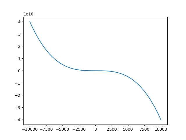
Ordinary cubic polynomial regression models are as follows (python grammatical expression):

y = a0 + a1 * x + a2 * (x**2) + a3 * (x**3) + e

When a0,a1,a2,a3,e = 10,-0.2,-0.03,-0.04,0.5, the general figures are as follows:

The source code is as follows:

#! /usr/bin/env python
#-*- coding:utf-8 -*-
import pylab
import pandas as pd

def fun(x):
    # y = a0 + a1 * x + a2 * (x**2) + a3 * (x**3)+ e
    a0,a1,a2,a3,e = 10,-0.2,-0.03,-0.04,0.5
    y = a0 + a1 * x + a2 * (x**2) + a3 * (x**3)+ e
    return y

arrX = range(-10000,10000)
arrY = []

for x in arrX :
    arrY.append(fun(x))

pylab.plot(arrX,arrY)
pylab.show()

polynomial regression

In the single factor (continuous variable) test, when the regression function can not be described by a straight line, the non-linear regression function should be considered. Polynomial regression is a kind of non-linear regression. This refers to single-factor polynomial regression, that is, one-variable polynomial regression.

Generally, the non-linear regression function is unknown, or even if it is known, it may not be possible to transform a simple function transformation into a linear model. At this time, the usual practice is to use the factor polynomial. If the scatter plot shows that the regression function has a "bend", quadratic polynomial can be used; cubic polynomial can be used for two bends; quadratic polynomial can be used for three bends, and so on.

The real regression function may not be a polynomial of a certain number of times, but as long as it fits well, it is feasible to approximate the real regression function with appropriate polynomials.

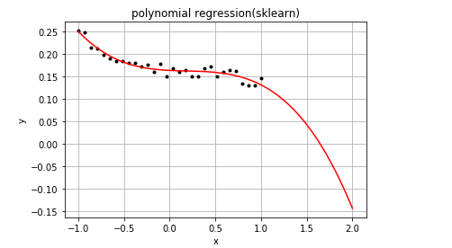
Using sklearn to Solve Polynomial Regression Problem

The sample code is as follows:

#! /usr/bin/env python
#-*- coding:utf-8 -*-
# polynomial regression
import matplotlib.pyplot as plt
import numpy as np
from sklearn.linear_model import LinearRegression
from sklearn.preprocessing import PolynomialFeatures

rng = np.random.RandomState(1)

def fun(x):
    a0,a1,a2,a3,e = 0.1,-0.02,0.03,-0.04,0.05
    y = a0 + a1 * x + a2 * (x**2) + a3 * (x**3)+ e
    y += 0.03 * rng.rand(1)
    return y

plt.figure()
plt.title('polynomial regression(sklearn)')
plt.xlabel('x')
plt.ylabel('y')
plt.grid(True)

X = np.linspace(-1, 1, 30)
arrY = [fun(x) for x in X]
X = X.reshape(-1,1)
y = np.array(arrY).reshape(-1,1)

plt.plot(X, y, 'k.')

qf = PolynomialFeatures(degree=3)
qModel = LinearRegression()
qModel.fit(qf.fit_transform(X), y)

X_predict = np.linspace(-1, 2, 100)
X_predict_result = qModel.predict(qf.transform(X_predict.reshape(X_predict.shape[0], 1)))
plt.plot(X_predict,X_predict_result , 'r-')

plt.show()

The code github address: https://github.com/mike-zhang/pyExamples/blob/master/algorithm/NonLinearRegression/pr_sklearn_test1.py

The operation results are as follows:

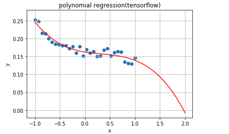
Using tensorflow to solve polynomial regression problem

The sample code is as follows:

#! /usr/bin/env python
#-*- coding:utf-8 -*-

import tensorflow as tf
import numpy as np
import matplotlib.pyplot as plt

learning_rate = 0.01
training_epochs = 40
rng = np.random.RandomState(1)

def fun(x):
    a0,a1,a2,a3,e = 0.1,-0.02,0.03,-0.04,0.05
    y = a0 + a1 * x + a2 * (x**2) + a3 * (x**3)+ e
    y += 0.03 * rng.rand(1)
    return y


trX = np.linspace(-1, 1, 30)
arrY = [fun(x) for x in trX]
num_coeffs = 4
trY = np.array(arrY).reshape(-1,1)

X = tf.placeholder("float")
Y = tf.placeholder("float")

def model(X, w):
    terms = []
    for i in range(num_coeffs):
        term = tf.multiply(w[i], tf.pow(X, i))
        terms.append(term)
    return tf.add_n(terms)

w = tf.Variable([0.] * num_coeffs, name="parameters")
y_model = model(X, w)

cost = tf.reduce_sum(tf.square(Y-y_model))
train_op = tf.train.GradientDescentOptimizer(learning_rate).minimize(cost)

with tf.Session() as sess :
    init = tf.global_variables_initializer()
    sess.run(init)

    for epoch in range(training_epochs):
        for (x, y) in zip(trX, trY):
            sess.run(train_op, feed_dict={X: x, Y: y})

    w_val = sess.run(w)
    print(w_val)

plt.figure()
plt.xlabel('x')
plt.ylabel('y')
plt.grid(True)
plt.title('polynomial regression(tensorflow)')
plt.scatter(trX, trY)
trX2 = np.linspace(-1, 2, 100)
trY2 = 0
for i in range(num_coeffs):
    trY2 += w_val[i] * np.power(trX2, i)
plt.plot(trX2, trY2, 'r-')
plt.show()