Reproduced from: https://blog.csdn.net/JAVA528416037/article/details/91998019
brief introduction
PostgreSQL is "the most advanced open source relational database in the world". Because of the late appearance, the customer base is less than MySQL, but the momentum of development is very strong, the biggest advantage is completely open source.
MySQL is the most popular open source relational database in the world. At present, the customer base is large. With the acquisition of Oracle, the degree of open source decreases. Especially recently, the free MariaDB branch has been pulled alone, which indicates that MySQL tends to be closed source.
As for the merits and demerits of the two, this is not the focus of this article. In general, there is no big difference. Next, we will only discuss the implementation plan in PG.
Implementation Plan
In the process of Query Planning path, different execution schemes of query requests are expressed by establishing different paths. After generating more qualified paths, the path with the least cost should be selected from them, which can be transformed into an execution plan and passed to the executor for execution. So how to generate the least-cost plan? Statistical information is used to estimate the cost of each node in the plan, and the related parameters are as follows:
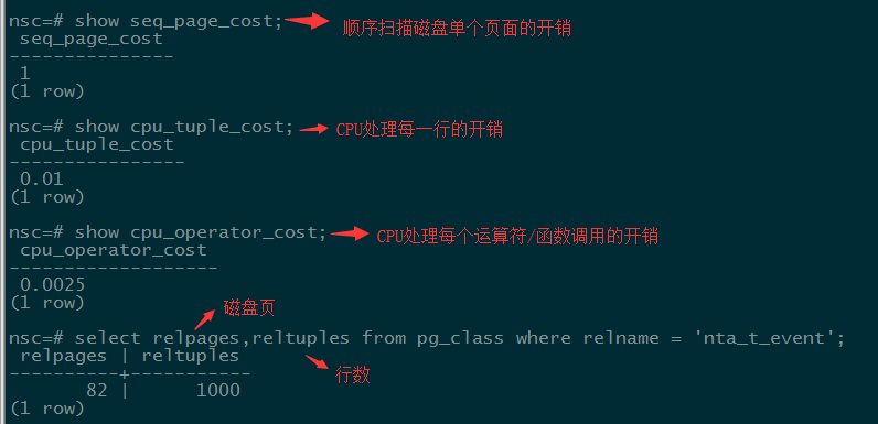
Calculate the cost:
# Estimated cost:
total_cost = seq_page_cost * relpages + cpu_tuple_cost *  reltuples


# Sometimes we don't want to use the default execution plan of the system. At this time, we can enforce control of the execution plan by forbidding/opening the grammar of some operation:
enable_bitmapscan = on
enable_hashagg = on
enable_hashjoin = on
enable_indexscan = on #Index Scanning
enable_indexonlyscan = on #Read-Only Index Scanning
enable_material = on #Materialized view
enable_mergejoin = on
enable_nestloop = on
enable_seqscan = on
enable_sort = on
enable_tidscan = on

# According to the scanning mode above and filtering cost:
Cost = seq_page_cost * relpages + cpu_tuple_cost *  reltuples + cpu_operation_cost * reltuples
Each SQL statement has its own execution plan. We can use the explain instruction to get the execution plan. The grammar is as follows:
nsc=# \h explain;
Command: EXPLAIN
Description: show the execution plan of a statement
Syntax:
EXPLAIN [ ( option [, ...] ) ] statement
EXPLAIN [ ANALYZE ] [ VERBOSE ] statement
where option can be one of:
ANALYZE [ boolean ] -- Whether it is really implemented by default false
VERBOSE [ boolean ] -- Whether to display details, default false
COSTS [ boolean ] -- Whether to display cost information, default true
BUFFERS [ boolean ] -- Whether to display cache information, default false,Pre-event is analyze
TIMING [ boolean ] -- Whether to display time information
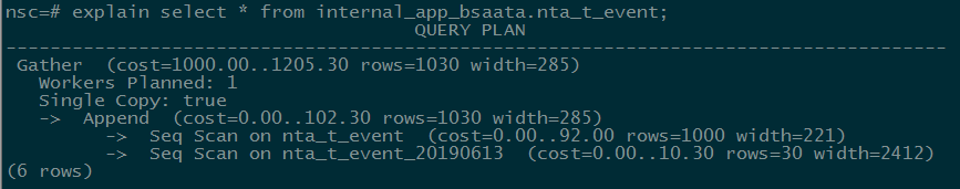
FORMAT { TEXT | XML | JSON | YAML } -- Input format, default is textAs shown in the figure below, cost is an important indicator. cost=1000.00..1205.30. The cost of executing SQL is divided into two parts. The first part represents the start time (startup) of 1000 ms, and the second part represents the total time (total) of 1205.30 ms, which is the cost of executing the whole SQL. Rows represent the number of predicted rows, which may differ from the actual number of records. The database often vacuum or analyze, and the closer the value is to the actual value. The total width of all fields representing the query results is 285 bytes.
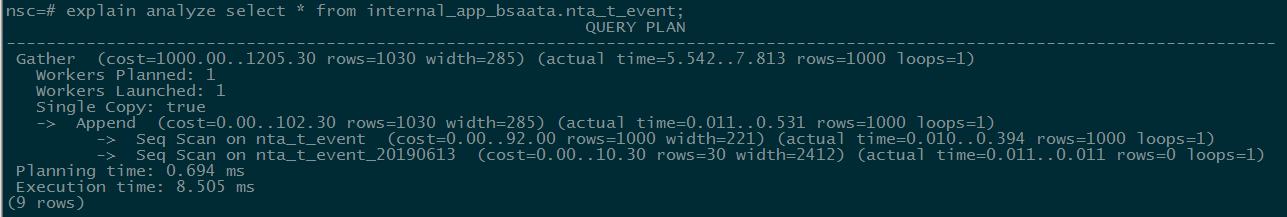
You can add the analyze keyword after explain ing to get the real execution plan and execution time by executing the SQL. The first number in the actual time represents the time required to return the first line, and the second number represents the time taken to execute the entire sql. Loops is the number of loops for the node. When loops are greater than 1, the total cost is: actual time * loops.
Execution Planning Node Type
In the execution plan of PostgreSQL, it is read from top to bottom. Usually, the execution plan has relevant index to represent different plan nodes. There are four types of plan nodes: Control Node, Scan Node, Materialization Node, Join Nod. E).
Control node: append, an execution node that organizes multiple word tables or sub-queries, is mainly used for union operations.
Scanning Node: Used to scan objects such as tables for tuples
Seq Scan: Read all the data blocks of the table from beginning to end, and select the eligible data blocks.
Index Scan: In order to speed up the query, find the physical location of the required data rows in the index, and then read out the corresponding data in the table data block, such as B tree, GiST, GIN, BRIN, HASH.
Bitmap Index/Heap Scan (Bitmap Index/Result Scan): Build a bitmap in memory for the qualified rows or blocks. After scanning the index, read the corresponding data according to the data file of the bitmap list. First, find the qualified rows in the index through Bitmap Index Scan, and build a bitmap in memory. Then scan Bitmap Heap Scan in the table.
Physical Node: Can cache the execution results into the cache, that is, the result tuple cache generated when the first execution, waiting for the upper node to use. For example, the sort node can get all tuples returned by the lower node and sort them according to the specified attributes, and cache the ranking results. Every time the upper node takes tuple, it slows down. Read on demand in storage.
Materialize: Caching tuples returned by lower-level nodes (such as when joining tables)
Sort: Sort the nodes returned from the lower layer (if memory exceeds the specified size of the iwork_mem parameter, the workspace of the node switches to temporary files, resulting in a dramatic performance degradation)
Group: Group operations on lower-level sorting tuples
Agg: Execute aggregation functions (sum/max/min/avg)
Conditional filtering usually adds filtering conditions after where. When scanning data rows, the rows satisfying filtering conditions will be found. Conditional filtering displays Filter in the execution plan. If there is an index on the column of condition, it may go indexing, but it will not go through filtering.
Connecting Nodes: Connecting operations in relational algebra can be implemented in a variety of ways (conditional connection/left connection/right connection/full connection/natural connection)
Nestedloop Join: The inner table is driven by the outer table. Every row returned by the outer table must search for the matching row in the inner table, so the result set returned by the whole query can not be too large. The table returned with a smaller subset should be regarded as the outer table, and the join field of the inner table should be indexed. The execution process is to determine one outer table and another inner table, each row of which is associated with the corresponding record in the inner table.
Hash Join: The optimizer uses two comparative tables and uses join attributes to create hash tables in memory, then scans larger tables and detects hash tables to find rows that match hash tables.
Merge Join: Usually hash connections perform better than merge connections, but if the source data is indexed or the results have been sorted, merge connections perform better than hash connections.
Explain
| Operational type | Operational instructions | Is there a start-up time? |
| Seq Scan | Sequential Scanning Table | No startup time |
| Index Scan | Index Scanning | No startup time |
| Bitmap Index Scan | Index Scanning | Start-up time |
| Bitmap Heap Scan | Index Scanning | Start-up time |
| Subquery Scan | Subquery | No startup time |
| Tid Scan | Line Number Retrieval | No startup time |
| Function Scan | Function Scanning | No startup time |
| Nested Loop Join | nested loops join | No startup time |
| Merge Join | Merge connection | Start-up time |
| Hash Join | HASH join | Start-up time |
| Sort | Order by | Start-up time |
| Hash | Hashing Operation | Start-up time |
| Result | Function scanning, independent of specific tables | No startup time |
| Unique | distinct/union | Start-up time |
| Limit | limit/offset | Start-up time |
| Aggregate | Aggregation functions such as count, sum,avg | Start-up time |
| Group | group by | Start-up time |
| Append | union operation | No startup time |
| Materialize | Subquery | Start-up time |
| SetOp | intersect/except | Start-up time |
Explanation of examples
Slow sql is as follows:
SELECT
	te.event_type,
	sum(tett.feat_bytes) AS traffic
FROM t_event te
LEFT JOIN t_event_traffic_total tett
ON tett.event_id = te.event_id
WHERE
	((te.event_type >= 1 AND te.event_type <= 17) OR (te.event_type >= 23 AND te.event_type <= 26) OR (te.event_type >= 129 AND te.event_type <= 256))
AND te.end_time >= '2017-10-01 09:39:41+08:00'
AND te.begin_time <= '2018-01-01 09:39:41+08:00'
AND tett.stat_time >= '2017-10-01 09:39:41+08:00'
AND tett.stat_time < '2018-01-01 09:39:41+08:00'
GROUP BY te.event_type
ORDER BY total_count DESC
LIMIT 10
Time-consuming: about 4 seconds
Function: Event tables are associated with event flow tables to identify TOP10 event types arranged by total traffic size over a period of time
Number of records:
select count(1) from t_event;  -- 535881 strip
select count(1) from t_event_traffic_total; -- 2123235 strip
Result:
event_type    traffic
17	2.26441505638877E17
2	2.25307250128674E17
7	1.20629298837E15
26	285103860959500
1	169208970599500
13	47640495350000
6	15576058500000
3	12671721671000
15	1351423772000
11	699609230000
Implementation plan:
Limit  (cost=5723930.01..5723930.04 rows=10 width=12) (actual time=3762.383..3762.384 rows=10 loops=1)
  Output: te.event_type, (sum(tett.feat_bytes))
  Buffers: shared hit=1899 read=16463, temp read=21553 written=21553
  ->  Sort  (cost=5723930.01..5723930.51 rows=200 width=12) (actual time=3762.382..3762.382 rows=10 loops=1)
        Output: te.event_type, (sum(tett.feat_bytes))
        Sort Key: (sum(tett.feat_bytes))
        Sort Method: quicksort  Memory: 25kB
        Buffers: shared hit=1899 read=16463, temp read=21553 written=21553
        ->  HashAggregate  (cost=5723923.69..5723925.69 rows=200 width=12) (actual time=3762.360..3762.363 rows=18 loops=1)
              Output: te.event_type, sum(tett.feat_bytes)
              Buffers: shared hit=1899 read=16463, temp read=21553 written=21553
              ->  Merge Join  (cost=384982.63..4390546.88 rows=266675361 width=12) (actual time=2310.395..3119.886 rows=2031023 loops=1)
                    Output: te.event_type, tett.feat_bytes
                    Merge Cond: (te.event_id = tett.event_id)
                    Buffers: shared hit=1899 read=16463, temp read=21553 written=21553
                    ->  Sort  (cost=3284.60..3347.40 rows=25119 width=12) (actual time=21.509..27.978 rows=26225 loops=1)
                          Output: te.event_type, te.event_id
                          Sort Key: te.event_id
                          Sort Method: external merge  Disk: 664kB
                          Buffers: shared hit=652, temp read=84 written=84
                          ->  Append  (cost=0.00..1448.84 rows=25119 width=12) (actual time=0.027..7.975 rows=26225 loops=1)
                                Buffers: shared hit=652
                                ->  Seq Scan on public.t_event te  (cost=0.00..0.00 rows=1 width=12) (actual time=0.001..0.001 rows=0 loops=1)
                                      Output: te.event_type, te.event_id
                                      Filter: ((te.end_time >= '2017-10-01 09:39:41+08'::timestamp with time zone) AND (te.begin_time <= '2018-01-01 09:39:41+08'::timestamp with time zone) AND (((te.event_type >= 1) AND (te.event_type <= 17)) OR ((te.event_type >= 23) AND (te.event_type <= 26)) OR ((te.event_type >= 129) AND (te.event_type <= 256))))
                                ->  Scanning sub-table process, omitting...
                    ->  Materialize  (cost=381698.04..392314.52 rows=2123296 width=16) (actual time=2288.881..2858.256 rows=2123235 loops=1)
                          Output: tett.feat_bytes, tett.event_id
                          Buffers: shared hit=1247 read=16463, temp read=21469 written=21469
                          ->  Sort  (cost=381698.04..387006.28 rows=2123296 width=16) (actual time=2288.877..2720.994 rows=2123235 loops=1)
                                Output: tett.feat_bytes, tett.event_id
                                Sort Key: tett.event_id
                                Sort Method: external merge  Disk: 53952kB
                                Buffers: shared hit=1247 read=16463, temp read=21469 written=21469
                                ->  Append  (cost=0.00..49698.20 rows=2123296 width=16) (actual time=0.026..470.610 rows=2123235 loops=1)
                                      Buffers: shared hit=1247 read=16463
                                      ->  Seq Scan on public.t_event_traffic_total tett  (cost=0.00..0.00 rows=1 width=16) (actual time=0.001..0.001 rows=0 loops=1)
                                            Output: tett.feat_bytes, tett.event_id
                                            Filter: ((tett.stat_time >= '2017-10-01 09:39:41+08'::timestamp with time zone) AND (tett.stat_time < '2018-01-01 09:39:41+08'::timestamp with time zone))
                                      ->  Scanning sub-table process, omitting...
Total runtime: 3771.346 ms
Interpretation of the implementation plan:
Line 40 - > 30: Scan the t_event_traffic_total table sequentially through the index created on the end time, filter out the eligible data according to the time span of three months, totaling 2123235 records.
Line 26 - > 21: According to the time, 26225 qualified records in t_event table were filtered out.
Line 30 - > 27: sort by traffic size.
Line 12 - > 09: Two tables perform join operation and complete 200 records;
Line 08 - > 04: Sort the final 200 records by size;
Line 01: Execute limit to take 10 records.
The longest time spent in the whole execution plan is to filter the t_event_traffic_total table according to the time condition. Because there are more vocabularies and more records, it will cost 2.8s. So the idea of our optimization is relatively simple. According to the actual time, we can check whether there are indexes in the table directly and spend more subtables. Not many, there is no room for optimization, and after investigation, found that a sub-table of data amounted to 153,1147.
Welcome to Technical Public: Architect Growth Camp
