
R and statistics, R language and statistics are a pair of brothers. It's hard to leave each other!
Here is a record of what I didn't know before in this book. Welcome to communicate with me! Vector pattern, the author wrote a function to do this. I'll learn and climb on the shoulders of giants. As I understand it, this is equivalent to motif, the element with the most counts.
mode <- function(x) {
  temp <- table(x)
  names(temp)[temp == max(temp)]
}
3.5 multivariate correlation analysis in R
In order to avoid the negative impact of a single variable, the following is the process of multivariate correlation analysis shown by correlation matrix and covariance:
# Multivariate linear correlation
data("mtcars")
# Covariance matrix (linear correlation)
cov(mtcars[1:3])
# mpg cyl disp
# mpg 36.324103 -9.172379 -633.0972
# cyl -9.172379 3.189516 199.6603
# disp -633.097208 199.660282 15360.7998
# Correlation matrix (degree of correlation)
cor(mtcars[1:3])
# mpg cyl disp
# mpg 1.0000000 -0.8521620 -0.8475514
# cyl -0.8521620 1.0000000 0.9020329
# disp -0.8475514 0.9020329 1.0000000
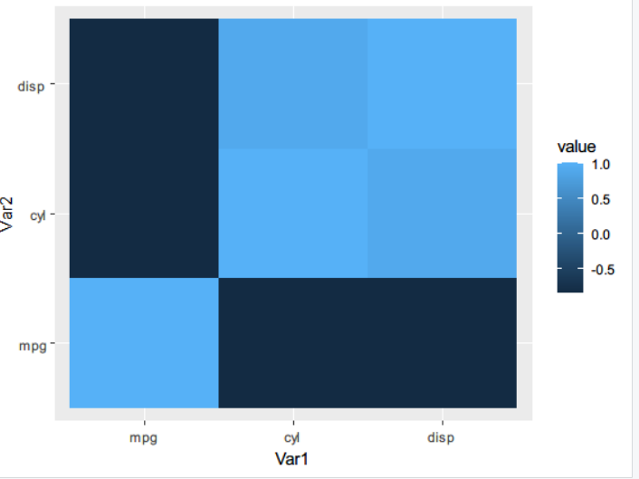
# Correlation matrix thermodynamic diagram
library(reshape2)
library(ggplot2)
qplot(x=Var1, y=Var2, data=melt(cor(mtcars[1:3])), fill=value, geom='tile')
3.6 multiple regression analysis
Evaluate the correlation between independent and non independent variables
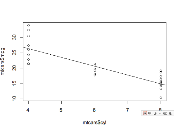
# regression
lmfit <- lm(mtcars$mpg ~ mtcars$cyl)
lmfit
# Call:
#   lm(formula = mtcars$mpg ~ mtcars$cyl)
#
# Coefficients:
#   (Intercept)   mtcars$cyl
# 37.885       -2.876
summary(lmfit) #More detailed information?
# Call:
#   lm(formula = mtcars$mpg ~ mtcars$cyl)
#
# Residuals:
#   Min      1Q  Median      3Q     Max
# -4.9814 -2.1185  0.2217  1.0717  7.5186
#
# Coefficients:
#   Estimate Std. Error t value Pr(>|t|)
# (Intercept)  37.8846     2.0738   18.27  < 2e-16 ***
#   mtcars$cyl   -2.8758     0.3224   -8.92 6.11e-10 ***
#   ---
#   Signif. codes:  0 '***' 0.001 '**' 0.01 '*' 0.05 '.' 0.1 ' ' 1
#
# Residual standard error: 3.206 on 30 degrees of freedom
# Multiple R-squared:  0.7262, Adjusted R-squared:  0.7171
# F-statistic: 79.56 on 1 and 30 DF,  p-value: 6.113e-10
# Drawing
plot(mtcars$cyl,mtcars$mpg)
abline(lmfit)
A slightly ugly picture was born.
F statistics can produce an F statistic, which is the ratio of the mean square and mean square error of the model. Therefore, when the F statistic is large, it means that the original hypothesis is rejected and the regression model has the ability to predict.
3.7 perform binomial distribution test
It is proved that the hypothesis is not established accidentally, but has statistical significance.
Binomial distribution test
library(stats)
binom.test(x=92,n=315,p=1/6)
 Exact binomial test

data:  92 and 315
number of successes = 92, number of trials = 315, p-value = 3.458e-08
alternative hypothesis: true probability of success is not equal to 0.1666667
95 percent confidence interval:
 0.2424273 0.3456598
sample estimates:
probability of success
             0.2920635
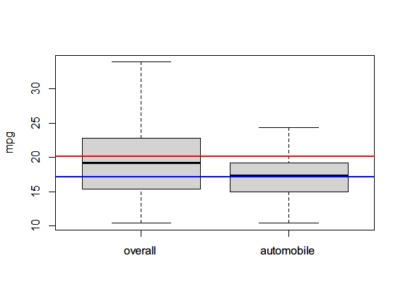
3.8 perform t-test
boxplot(mtcars$mpg, mtcars$mpg[mtcars$am==0], ylab="mpg", name=c("overall", "automobile"))
abline(h=mean(mtcars$mpg), lwd=2, col="red")
abline(h=mean(mtcars$mpg[mtcars$am==0]), lwd=2, col="blue")
t.test(mtcars$mpg~mtcars$am)
#########################
 Welch Two Sample t-test

data:  mtcars$mpg by mtcars$am
t = -3.7671, df = 18.332, p-value = 0.001374
alternative hypothesis: true difference in means is not equal to 0
95 percent confidence interval:
 -11.280194  -3.209684
sample estimates:
mean in group 0 mean in group 1
       17.14737        24.39231
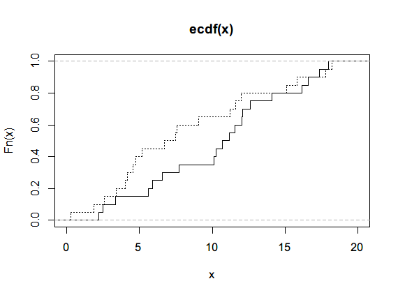
3.9 Kolmogorov Smirnov test
Single sample test is used to compare whether the samples conform to a known sequence (similarity of continuous probability distribution), and double sample test is used to compare the cumulative distribution of two data sets.
# Single sample
x <- rnorm(50)
ks.test(x,'pnorm')
###################
 One-sample Kolmogorov-Smirnov test

data:  x
D = 0.09625, p-value = 0.707
alternative hypothesis: two-sided
# Two samples, empirical distribution function, ecdf
set.seed(3)
x<- runif(n=20, min=0,max=20)
y<- runif(n=20, min=0,max=20)
par(new=TRUE)
plot(ecdf(x), do.points=FALSE, verticals = T, xlim=c(0,20))
lines(ecdf(y), do.points=FALSE, verticals = T, lty=3)
ks.test(x,y)
##############
 Two-sample Kolmogorov-Smirnov test

data:  x and y
D = 0.3, p-value = 0.3356
alternative hypothesis: two-sided
Both p values are greater than 0.05, and the original hypothesis is true.
3.10 Wilcoxon rank sum test and Wilcoxon signed rank test
Nonparametric test does not need to assume that the samples obey normal distribution
> wilcox.test(mtcars$mpg~mtcars$am,data=mtcars)

 Wilcoxon rank sum test with continuity correction
#############
data:  mtcars$mpg by mtcars$am
W = 42, p-value = 0.001871
alternative hypothesis: true location shift is not equal to 0

Warning message:
In wilcox.test.default(x = c(21.4, 18.7, 18.1, 14.3, 24.4, 22.8,  :
  Cannot accurately calculate linked p value
The knotting prompt is because there are duplicate values, and the p value is less than 0.05. The original hypothesis is not tenable, and the mpg distribution of automatic and manual vehicles is different.
3.11 Pearson chi square test
> ftable <- table(mtcars$am, mtcars$gear)
> ftable
   ##############
     3  4  5
  0 15  4  0
  1  0  8  5
mosaicplot(ftable, main="Mosaic diagram of manual and automatic front drive gears", color=TRUE)
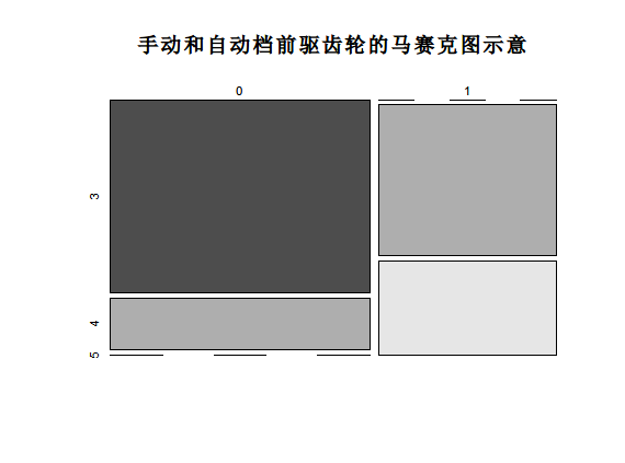
Pearson test must ensure that the input samples meet the following two conditions: first, the input data set must be category data; Second, the variable must contain two or more independent data groups.
R also provides users with other hypothesis testing methods:
- 1. Percentage inspection prop Test: used to test whether the percentage distribution of different sample sets is consistent.
- 2.Z Test (simple.z.test in UsingT package): compare the sample mean with the mean and standard deviation of the overall data set.
- 3.Bartlett test: test whether the variance of different data sets is consistent
- 4. Kruskal Wallis rank sum test (kruskal.test): judge whether the distribution of the data set is consistent under the premise of uncertain whether the data set obeys the normal distribution.
- 5. Shapiro Wilk test: used for normality test.
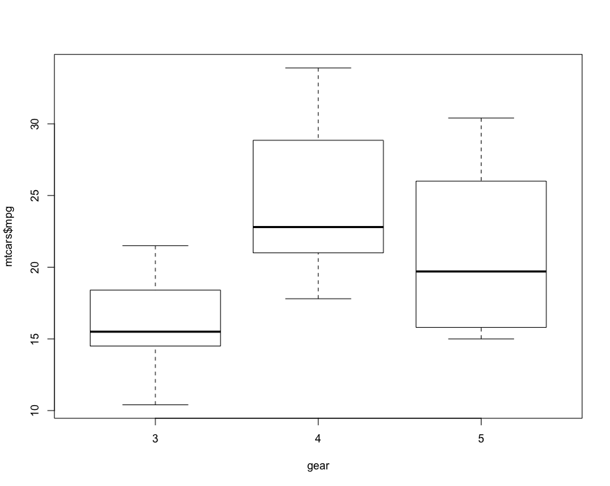
3.12 one way ANOVA
ANOVA (Analysis of Variance) is used to find the association between category independent variables and continuous non independent variables, mainly to test whether the mean value is the same. If only one category variable is included as an independent variable, one-way ANOVA is used. Otherwise, if two or more category variables are included, two-way ANOVA is required.
# First, visualization
boxplot(mtcars$mpg~factor(mtcars$gear),xlab = 'gear', y='mpg')
# Then, one-way ANOVA
oneway.test(mtcars$mpg~factor(mtcars$gear))
###################The advantage of this method is that Welch correction is applied to deal with the non-uniformity of variables
 One-way analysis of means (not assuming equal variances)

data:  mtcars$mpg and factor(mtcars$gear)
F = 11.285, num df = 2.0000, denom df = 9.5083, p-value = 0.003085
# aov is also OK, and the returned result is more non rich
summary(aov(mtcars$mpg~as.factor(mtcars$gear)))
##################
                       Df Sum Sq Mean Sq F value   Pr(>F)
as.factor(mtcars$gear)  2  483.2  241.62    10.9 0.000295 ***
Residuals              29  642.8   22.17
---
Signif. codes:  0 '***' 0.001 '**' 0.01 '*' 0.05 '.' 0.1 ' ' 1
# The model generated by the aov function can also enter the summary in the form of a table
model.tables(aov(mtcars$mpg~as.factor(mtcars$gear)))
# ############
Tables of effects

 as.factor(mtcars$gear)
         3      4     5
    -3.984  4.443 1.289
rep 15.000 12.000 5.000
# TukeyHSD post hoc comparison test (multiple comparison test)
TukeyHSD(aov(mtcars$mpg~as.factor(mtcars$gear)))
# ##############
  Tukey multiple comparisons of means
    95% family-wise confidence level

Fit: aov(formula = mtcars$mpg ~ as.factor(mtcars$gear))

$`as.factor(mtcars$gear)`
         diff        lwr       upr     p adj
4-3  8.426667  3.9234704 12.929863 0.0002088
5-3  5.273333 -0.7309284 11.277595 0.0937176
5-4 -3.153333 -9.3423846  3.035718 0.4295874
F-score is the ratio of inter group variance and intra group variance. If the overall significance level of F-test is large, it can be further post test. The most commonly used methods are Scheffe, Tukey Kramer method and Bonferroni correction.
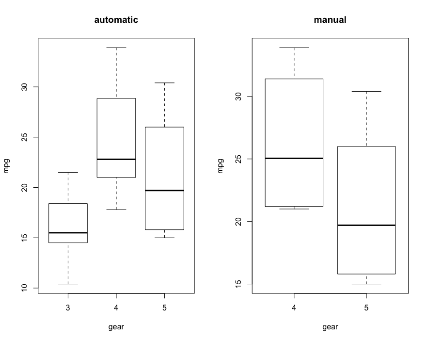
3.13 two way ANOVA
# Also visualize first
par(mfrow=c(1,2))
boxplot(mtcars$mpg~mtcars$gear, subset = (mtcars$am==0), xlab = 'gear', ylab = 'mpg', main='automatic')
boxplot(mtcars$mpg~mtcars$gear, subset = (mtcars$am==1), xlab = 'gear', ylab = 'mpg', main='manual')
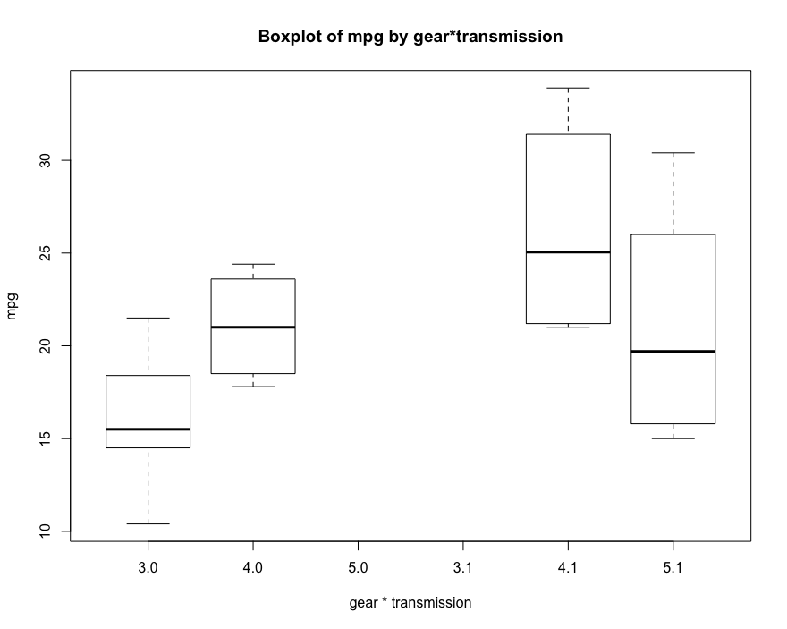
# Box diagram of correlation analysis between front drive gear * speed change mode and mpg
boxplot(mtcars$mpg~factor(mtcars$gear)*factor(mtcars$am), xlab = 'gear * transmission', ylab = 'mpg', main='Boxplot of mpg by gear*transmission')
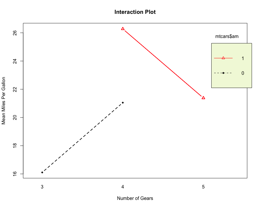
# Interaction graph to express the relationship between variables
interaction.plot(mtcars$gear, mtcars$am, mtcars$mpg, type = 'b',col = c(1:3), leg.bty = 'o',leg.bg = 'beige',lwd=2, pch = c(18,24,22),
main = "Interaction Plot")
# Two factor analysis of variance
summary(aov(mtcars$mpg~factor(mtcars$gear)*factor(mtcars$am)))
# #################
Df Sum Sq Mean Sq F value Pr(>F)
factor(mtcars$gear) 2 483.2 241.62 11.869 0.000185 ***
factor(mtcars$am) 1 72.8 72.80 3.576 0.069001 .
Residuals 28 570.0 20.36
---
Signif. codes: 0 '***' 0.001 '**' 0.01 '*' 0.05 '.' 0.1 ' ' 1
# Post Hoc Tests
TukeyHSD(aov(mtcars$mpg~factor(mtcars$gear)*factor(mtcars$am)))
# ###############
Tukey multiple comparisons of means
95% family-wise confidence level
Fit: aov(formula = mtcars$mpg ~ factor(mtcars$gear) * factor(mtcars$am))
$`factor(mtcars$gear)`
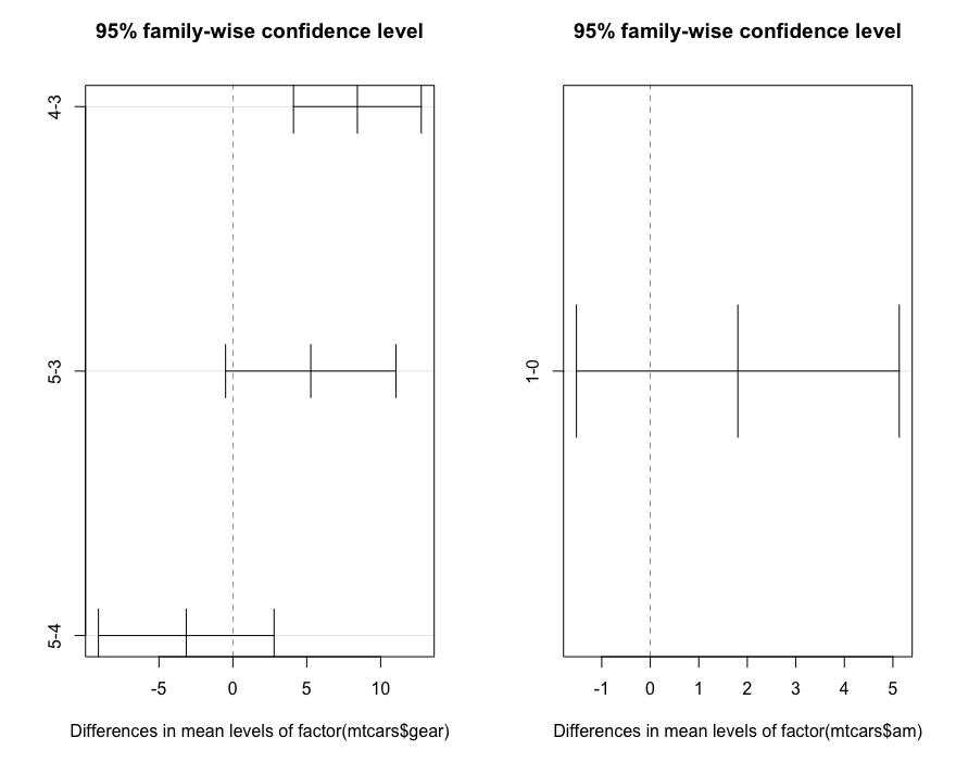
diff lwr upr p adj
4-3 8.426667 4.1028616 12.750472 0.0001301
5-3 5.273333 -0.4917401 11.038407 0.0779791
5-4 -3.153333 -9.0958350 2.789168 0.3999532
$`factor(mtcars$am)`
diff lwr upr p adj
1-0 1.805128 -1.521483 5.13174 0.2757926
par(mfrow=c(1,2))
plot(TukeyHSD(aov(mtcars$mpg~factor(mtcars$gear)*factor(mtcars$am))))
The extended function manova is suitable for multivariate analysis to test the influence of multivariate independent variables on multivariate non independent variables.