[Kaggle] Telco Customer Churn Telecom user churn prediction case
Part III introduction
in the second part of the case, we introduce in detail the common feature transformation methods, some of which are necessary for model training, such as natural number coding and unique heat coding, while some methods focus on improving data quality and are used as alternative methods for model optimization most of the time, such as continuous variable bin division, data standardization, etc. Of course, after that, we first try to build some models with strong interpretability to predict user churn, that is, we use logistic regression and decision tree model to predict user churn, and introduce the tuning skills of the two models in practice in detail. After the final model training is completed, We also focus on the interpretation methods of the modeling results of two interpretable models.
theoretically, the discrimination ability of tree model is stronger than that of logistic regression, but in the final modeling results of the previous section, we found that there is no significant difference between the modeling of the two models, and the prediction accuracy remains between 79% - 80%, which may indicate that many sample decision tree models that cannot be correctly discriminated by logistic regression can not be discriminated. Therefore, we speculate that, This is a data set that is "easy to get started and difficult to master". Of course, if we further try other "stronger" integrated learning algorithms, such as random forest, XGB, CatBoost, etc., the modeling results and logistic regression on the current data set are not much different. Therefore, we urgently need to further improve the quality of the data set through feature engineering method, so as to improve the final model effect.
of course, even if the complex model shows a better effect on the current data set, improving the data quality by using feature engineering method is still an essential part of optimizing the modeling results. As the popular description says, "the data quality determines the upper bound of the model, and the modeling process is only constantly approaching this upper bound", A series of methods to improve data quality in Feature Engineering, whether in industrial practice or in major top competitions, have become the most important means to improve the effect of the model.
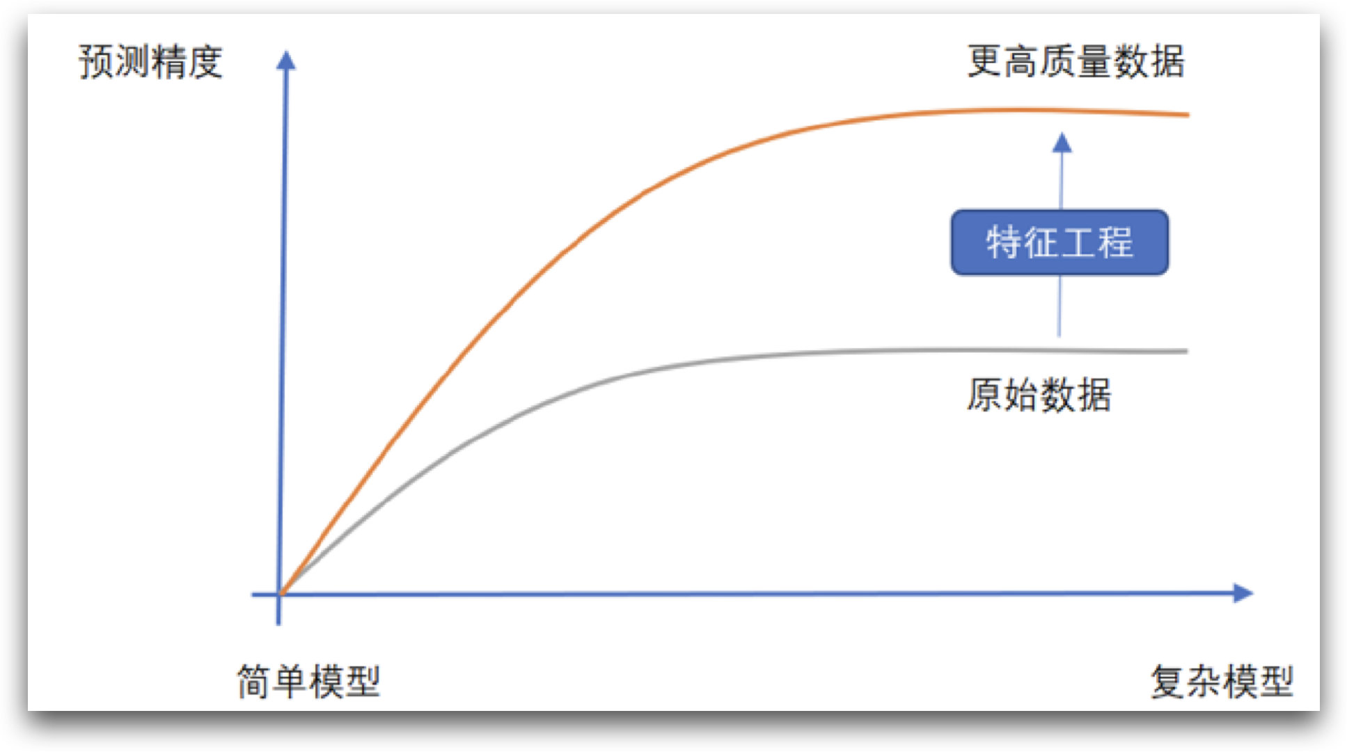
however, the so-called feature engineering method to improve data quality seems simple, but it is not easy to operate in practice. The difficulty lies not in the understanding of the specific operation methods. At least compared with the principle of machine learning algorithm, many methods of feature engineering are not complex. The biggest difficulty of Feature Engineering lies in the selection of methods in cooperation with models and data, as well as the engineering deployment and implementation of various methods. On the one hand, there are many feature engineering methods, which need to "adjust measures to local conditions" according to the actual situation, but the situation of data is changeable. Many times, it is necessary to combine the data exploration conclusion, the modeler's own experience and the familiarity with various alternative methods at the same time, so as to quickly formulate effective feature engineering strategies; On the other hand, unlike machine learning algorithms, many feature engineering methods have ready-made libraries that can be called directly. Many methods, especially some customized methods around the current data set, need to be implemented manually, and this process puts forward higher requirements for the modeler's own coding ability and engineering deployment ability. In a word, feature engineering is a highly relevant technology in practice, which is why the course introduces the common methods of Feature Engineering simultaneously in the process of introducing cases.
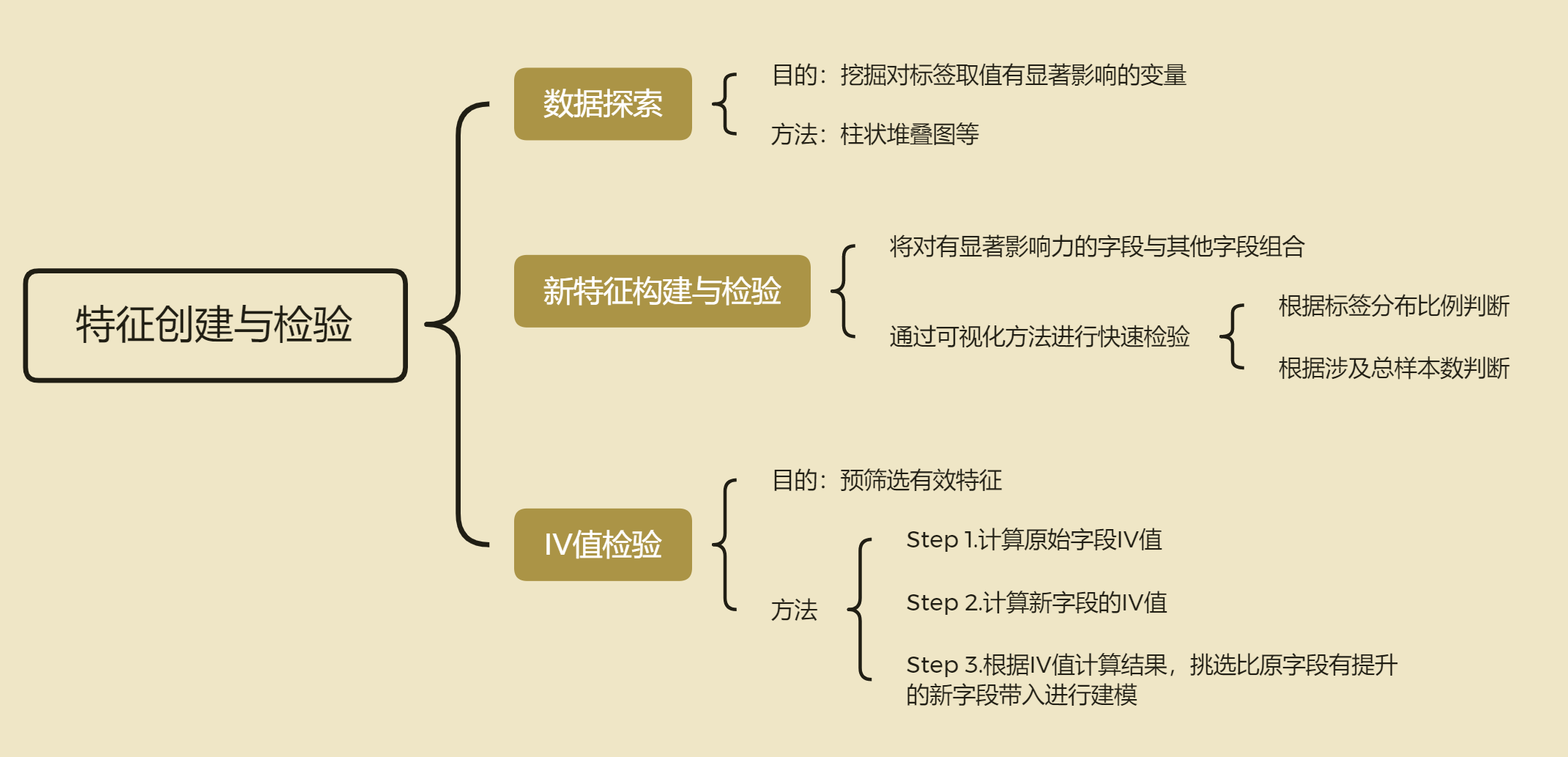
of course, from a broad perspective, all data adjustment work around the dataset can be regarded as a part of Feature Engineering, including missing value filling, data coding, feature transformation, etc. previously introduced. These methods can actually improve the data quality to a certain extent. At the beginning of this section, We will spend a whole section discussing another kind of feature engineering methods: feature derivation and feature screening. This method provides more dimensions to capture data rules by creating more features, so as to improve the effect of the model. Of course, feature derivation is also recognized as the most effective method to significantly improve the quality of data sets.
Part 3. Feature derivation and feature screening
at the beginning of this stage, we will focus on feature derivation and feature screening methods in Feature Engineering, so as to further improve the effect of the model. First, the third-party libraries involved in the previous operations need to be imported uniformly:
# Basic data scientific operation Library
import numpy as np
import pandas as pd

# Visualization Library
import seaborn as sns
import matplotlib.pyplot as plt

# Time module
import time

# sklearn Library
# Data preprocessing
from sklearn import preprocessing
from sklearn.compose import ColumnTransformer

# Practical function
from sklearn.metrics import accuracy_score, recall_score, precision_score, f1_score, roc_auc_score
from sklearn.model_selection import train_test_split

# Common evaluator
from sklearn.pipeline import make_pipeline
from sklearn.linear_model import LogisticRegression
from sklearn import tree
from sklearn.tree import DecisionTreeClassifier

# Grid search
from sklearn.model_selection import GridSearchCV

# Custom evaluator support module
from sklearn.base import BaseEstimator, TransformerMixin

# Custom module
from telcoFunc import *

# re module correlation
import inspect, re
telcoFunc is a user-defined module, in which previously customized functions and classes are saved, and subsequent newly added functions and classes will also be written into it step by step. telcoFunc Py file is provided with the courseware. It needs to be placed in the same folder as the current ipy file before it can be imported normally.
next, import the data and perform the data cleaning steps in Part 1.
# Read data
tcc = pd.read_csv('WA_Fn-UseC_-Telco-Customer-Churn.csv')

# Label continuous / discrete fields
# Discrete field
category_cols = ['gender', 'SeniorCitizen', 'Partner', 'Dependents',
                'PhoneService', 'MultipleLines', 'InternetService', 'OnlineSecurity', 'OnlineBackup',
                'DeviceProtection', 'TechSupport', 'StreamingTV', 'StreamingMovies', 'Contract', 'PaperlessBilling',
                'PaymentMethod']

# Continuous field
numeric_cols = ['tenure', 'MonthlyCharges', 'TotalCharges']

# label
target = 'Churn'

# ID column
ID_col = 'customerID'

# Verify whether the division can be completed
assert len(category_cols) + len(numeric_cols) + 2 == tcc.shape[1]

# Continuous field conversion
tcc['TotalCharges']= tcc['TotalCharges'].apply(lambda x: x if x!= ' ' else np.nan).astype(float)
tcc['MonthlyCharges'] = tcc['MonthlyCharges'].astype(float)

# Missing value filling
tcc['TotalCharges'] = tcc['TotalCharges'].fillna(0)

# Manual conversion of tag values
tcc['Churn'].replace(to_replace='Yes', value=1, inplace=True)
tcc['Churn'].replace(to_replace='No',  value=0, inplace=True)
features = tcc.drop(columns=[ID_col, target]).copy()
labels = tcc['Churn'].copy()
Next, you can directly bring in the data for feature derivation.
- Basic concepts and classification of feature derivation
the so-called feature derivation refers to the creation of new features through existing data. Feature derivation is sometimes called feature creation, feature extraction, etc. Generally speaking, there are two methods of feature derivation. One is to create new features according to the characteristics of the data set. At this time, feature derivation is actually a kind of unsupervised feature derivation. For example, add the two columns of monthly charges and total charges to create a new column; In another case, the label of data set is also taken into consideration to create new features. At this time, feature derivation is actually supervised feature derivation. As described in the previous section, continuous variables are boxed through the modeling results of decision tree (the column after boxed is also a new column created, but sometimes we will replace the original column). In most cases, feature derivation refers to unsupervised feature derivation, while supervised feature derivation is called target coding.
whether it is feature derivation or target coding, there are two ways to realize it. One is to synthesize artificial fields through in-depth data background and business background analysis. The fields created by this method often have strong business background and interpretability. At the same time, it will also improve the model effect more accurately and effectively, but the disadvantage is that the efficiency is slow, It requires manual analysis and screening. The second is to put aside the business background, directly create features in batch through some simple and violent engineering methods, and then select useful features from the massive feature pool for modeling. This method is simple and efficient, but the engineering method is seriously homogeneous, which is a necessary means in the competition, However, it is difficult to open the gap with other competitors who also use engineering means to create features in batches. Therefore, in practical application, it is often to create features in batches through engineering methods to improve the model effect, and then analyze the specific problems around the current modeling requirements, and try to manually create some fields to further improve the model effect.
of course, since we have conducted a certain degree of business background analysis and data exploration before, and considering the explanation order of code implementation difficulty from easy to difficult, we will first discuss the method of artificial field synthesis, and then introduce the method of engineering batch creation of words.
Part 3.1 artificial field synthesis
the so-called artificial field synthesis refers to the feature creation method based on manual judgment after a certain degree of data exploration and business analysis. The features created by this method often have a certain business background, and the method used in the creation process is uncertain. In many cases, the created fields can also be used as new business indicators. Of course, because there is no fixed process for artificial field synthesis, some "inspiration" is often needed. Next, we will conduct artificial field synthesis according to the data exploration and business analysis results of the previous two parts.
it should be emphasized that in the process of actual synthetic fields, it is often more difficult to find the right idea than engineering implementation, and the "idea" is often not fixed, and most of the time, the idea is highly related to practical experience. Therefore, the idea of synthetic features introduced in this section is not a "golden rule" similar to algorithm theory, but more like a summary based on long-term practical experience. At the same time, it should be emphasized that the idea is not invariable. In practical work or competition, students can also use the basic idea introduced in this section as a reference, Try more of your own understanding and ideas. In addition, each idea does not exist independently. Many times, we need to think from different angles. In any case, everything is subject to the final practical effect.
generally speaking, there are three ways to synthesize features. One is to take basic business as the starting point and use business experience and common sense to assist feature creation; The second is to take the data law as the starting point and take the exploratory analysis conclusion at the data level as the basis for creating features; The third is to take the modeling results as the starting point, focus on the analysis of the data characteristics of misclassified samples, and create new features accordingly. In this section, we will first focus on the practical process of the first two ideas, and then discuss how to create features according to the model modeling results after introducing batch feature creation in the next section.
1, Feature creation based on business background
1. Analysis ideas
we all know that the ultimate goal of machine learning algorithm is to mine the laws of effective data, but for all data, there are the objective facts described behind the data (review the data concept introduced at the beginning of the course: data is a number describing the state attributes or operation laws of objective objects). Long before the birth of machine learning algorithm, People analyze more based on historical experience, and the long-term historical experience gradually accumulates into the so-called business experience. Although many business experience can not be quantified, it can be used as a breakthrough for us to create features. For example, user churn is actually a very common business scenario. Generally speaking, the factors affecting user stickiness may include service experience, user habits, group preferences, user registration time, homogeneous competitive products and other factors. Therefore, we can add two new fields in the current data set to measure user stickiness, One is the identification of new users (specially marking the users who have accessed the network in the last 1-2 months), and the other is the number of services purchased by users.
- New user ID
we know that if the user's registration time is short, the stickiness to the product is relatively weak. In the data set, the tenure field is a field describing the user's network access time. In all values of this field, considering that the shortest renewal period is one month, there is a category of users that need to pay attention to, that is, the users who have accessed the network in the last 1-2 months: these users not only have a short network access time, Moreover, under the provisions of the payment cycle, such users are likely to leave the network next month after a short experience of products and services. Therefore, we might as well create a separate field to mark the users whose tenure field is 1.
It should be noted here that we cannot judge whether the user is currently off the network by the user's access time and the period of signing the contract. This problem involves the statistical period of the data set, which will be discussed in depth later.
- Number of services purchased
in addition, we can also calculate the number of services purchased by users. A simple judgment is that the more services purchased by users, the greater the user stickiness and the smaller the probability of user loss. We can measure the user stickiness by simply summarizing the total number of all service categories including value-added services purchased by each user as a new field.
2.new_customer feature creation
create a new here_ The customer field is used to indicate whether it is a new customer. We classify all users with tenure value of 1 as new users. This field is a 0 / 1 secondary classification field, and 1 indicates new users. The field creation process is as follows.
first determine the screening conditions:
# Screening conditions
new_customer_con = (tcc['tenure'] == 1)
new_customer_con
#0        True
#1       False
#2       False
#3       False
#4       False
#        ...
#7038    False
#7039    False
#7040    False
#7041    False
#7042    False
#Name: tenure, Length: 7043, dtype: bool
Then create the field
new_customer = (new_customer_con * 1).values
Of course, whether the addition of this field can improve the model effect can be tested simply by calculating the correlation between the field and the label. If the field has strong correlation with the label, the model effect will be improved after adding this field with a high probability. The correlation test can be completed in the following ways:
# Extract dataset labels
y = tcc['Churn'].values
y
#array([0, 0, 1, ..., 0, 1, 0], dtype=int64)
np.corrcoef(new_customer, y)
#array([[1.      , 0.247925],
#       [0.247925, 1.      ]])
It can be found that there is a positive correlation between the new field and the label, that is, the loss probability of new users is large, and the correlation coefficient of 0.24 belongs to a large value in all the correlation coefficient calculation results (for details, please review the correlation coefficient calculation results of all fields and labels in Part 1), which can be considered to be brought into this field for modeling.
For this data set, it can be inferred from the calculation results of the overall correlation coefficient that when the absolute value of the correlation coefficient is greater than 0.2, it belongs to the available field.
3.new_customer new field effect
next, we test the impact of new features on model training. In order to facilitate comparison, we first run the model results without new features, and then run the model with new features. Most of the time, new features are validated on one model and will be validated on other models. Therefore, in order to test the results more quickly, here we only validate the performance of new features on logistic regression, and the validation process of other models is similar.
- Original data training results
first, run the "complete body" of logistic regression model training and hyperparametric search in Part 2 on the data that does not bring in new features. According to the discussion in Part 2, this process can get the best effect of logistic regression in the current data set. At the same time, according to the discussion in Part 2, when taking the accuracy as the optimization index, the threshold movement will not actually work, In order to speed up the search process, the threshold moving search condition will be removed in the grid search in this section. The execution process is as follows:
# Extract dataset features
features = tcc.drop(columns=[ID_col, target]).copy()

# Partition dataset
X_train, X_test, y_train, y_test = train_test_split(features, y, test_size=0.3, random_state=21)

# Check whether the column is completely divided
assert len(category_cols) + len(numeric_cols) == X_train.shape[1]

# Set converter flow
logistic_pre = ColumnTransformer([
    ('cat', preprocessing.OneHotEncoder(drop='if_binary'), category_cols),
    ('num', 'passthrough', numeric_cols)
])

num_pre = ['passthrough', preprocessing.StandardScaler(), preprocessing.KBinsDiscretizer(n_bins=3, encode='ordinal', strategy='kmeans')]

# Instantiated logistic regression evaluator
logistic_model = logit_threshold(max_iter=int(1e8))

# Set up machine learning flow
logistic_pipe = make_pipeline(logistic_pre, logistic_model)

# Set hyper parameter space
logistic_param = [
    {'columntransformer__num':num_pre, 'logit_threshold__penalty': ['l1'], 'logit_threshold__C': np.arange(0.1, 1.1, 0.1).tolist(), 'logit_threshold__solver': ['saga']},
    {'columntransformer__num':num_pre, 'logit_threshold__penalty': ['l2'], 'logit_threshold__C': np.arange(0.1, 1.1, 0.1).tolist(), 'logit_threshold__solver': ['lbfgs', 'newton-cg', 'sag', 'saga']},
]

# Instantiate grid search evaluator
logistic_search_r1 = GridSearchCV(estimator = logistic_pipe,
                                  param_grid = logistic_param,
                                  scoring='accuracy',
                                  n_jobs = 12)

# Output time
s = time.time()
logistic_search_r1.fit(X_train, y_train)
print(time.time()-s, "s")

# Calculation and prediction results
result_df(logistic_search_r1.best_estimator_, X_train, y_train, X_test, y_test)
#42.66864991188049 s
logistic_search_r1.best_params_
#{'columntransformer__num': 'passthrough',
# 'logit_threshold__C': 0.30000000000000004,
# 'logit_threshold__penalty': 'l2',
# 'logit_threshold__solver': 'lbfgs'}
logistic_search_r1.best_score_
#0.8042596348884381
- Bring in new_customer feature training
then we consider bringing in new features for modeling, and test the final effect of the model under the same search process:
new_customer.reshape(-1,1)
#array([[1],
#       [0],
#       [0],
#       ...,
#       [0],
#       [0],
#       [0]])
# Add new_customer column
features['new_customer'] = new_customer.reshape(-1, 1)
y
#array([0, 0, 1, ..., 0, 1, 0])


# Data preparation
X_train, X_test, y_train, y_test = train_test_split(features, y, test_size=0.3, random_state=21)

# Check whether the column is completely divided
category_new = category_cols + ['new_customer']
assert len(category_new) + len(numeric_cols) == X_train.shape[1]

# Set converter flow
logistic_pre = ColumnTransformer([
    ('cat', preprocessing.OneHotEncoder(drop='if_binary'), category_new),
    ('num', 'passthrough', numeric_cols)
])

num_pre = ['passthrough', preprocessing.StandardScaler(), preprocessing.KBinsDiscretizer(n_bins=3, encode='ordinal', strategy='kmeans')]

# Instantiated logistic regression evaluator
logistic_model = logit_threshold(max_iter=int(1e8))

# Set up machine learning flow
logistic_pipe = make_pipeline(logistic_pre, logistic_model)

# Set hyper parameter space
logistic_param = [
    {'columntransformer__num':num_pre, 'logit_threshold__penalty': ['l1'], 'logit_threshold__C': np.arange(0.1, 1.1, 0.1).tolist(), 'logit_threshold__solver': ['saga']},
    {'columntransformer__num':num_pre,  'logit_threshold__penalty': ['l2'], 'logit_threshold__C': np.arange(0.1, 1.1, 0.1).tolist(), 'logit_threshold__solver': ['lbfgs', 'newton-cg', 'sag', 'saga']},
]

# Instantiate grid search evaluator
logistic_search = GridSearchCV(estimator = logistic_pipe,
                               param_grid = logistic_param,
                               scoring='accuracy',
                               n_jobs = 12)

# Output time
s = time.time()
logistic_search.fit(X_train, y_train)
print(time.time()-s, "s")

# Calculation and prediction results
result_df(logistic_search.best_estimator_, X_train, y_train, X_test, y_test)
#42.22627019882202 s
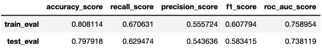
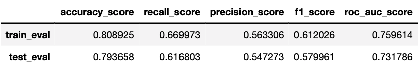
logistic_search.best_score_
#0.8054766734279919
it can be found that the average accuracy of the verification set of the model in grid search has increased from 0.8042 to 0.8052, about 0.1%, while the accuracy of the test set has increased from 0.793658 to 0.797918, about 0.3%, and the results also verify the effectiveness of the feature creation. At the same time, compared with the accuracy results of a single run of the training set, we found that the average accuracy rate of the verification set in the grid search can better represent the current generalization ability of the model (it is noted that the accuracy rate of a single run of the model with new features on the training set has decreased, but the accuracy rate on the test set has increased).
Generally speaking, in addition to some "masterstroke" feature creation, the feature creation that can improve the score on the thousandth percentile has achieved good results.
in addition, it should be noted here that in the process of feature derivation, since new features are created through other features, there is often strong collinearity between new and old features. In order to eliminate the impact of collinearity on the model effect, it is often necessary to bring it into the grid search process for model training.
logistic_search.best_params_
#{'columntransformer__num': 'passthrough',
# 'logit_threshold__C': 0.1,
# 'logit_threshold__penalty': 'l2',
# 'logit_threshold__solver': 'newton-cg'}
For highly collinear data sets, when training the logistic regression model, grid search can often find a set of parameters with greater structural risk weight to reduce the influence of collinearity and ensure the generalization ability of the model.
of course, running long pieces of code repeatedly each time will be slightly cumbersome. We can encapsulate the above verification process into a function to simplify the number of explicit code.
def features_test(new_features,
                  features = features,
                  labels = labels,
                  category_cols = category_cols,
                  numeric_cols = numeric_cols):
    """
    New feature test function

    :param features: Dataset characteristics
    :param labels: Dataset label
    :param new_features: New features
    :param category_cols: Discrete column name
    :param numeric_cols: Continuous column name
    :return: result_df Evaluation index
    """

    # Data preparation
    if type(new_features) == np.ndarray:
        name = 'new_features'
        new_features = pd.Series(new_features, name=name)
    # print(new_features)

    features = features.copy()
    category_cols = category_cols.copy()
    numeric_cols = numeric_cols.copy()

    features = pd.concat([features, new_features], axis=1)
    # print(features.columns)
    X_train, X_test, y_train, y_test = train_test_split(features, labels, test_size=0.3, random_state=21)

    # Partition continuous variable / discrete variable
    if type(new_features) == pd.DataFrame:
        for col in new_features:
            if new_features[col].nunique() >= 15:
                numeric_cols.append(col)
            else:
                category_cols.append(col)

    else:
        if new_features.nunique() >= 15:
            numeric_cols.append(name)
        else:
            category_cols.append(name)


    # print(category_cols)
    # Check whether the column is completely divided
    assert len(category_cols) + len(numeric_cols) == X_train.shape[1]

    # Set converter flow
    logistic_pre = ColumnTransformer([
        ('cat', preprocessing.OneHotEncoder(drop='if_binary'), category_cols),
        ('num', 'passthrough', numeric_cols)
    ])

    num_pre = ['passthrough', preprocessing.StandardScaler(), preprocessing.KBinsDiscretizer(n_bins=3, encode='ordinal', strategy='kmeans')]

    # Instantiated logistic regression evaluator
    logistic_model = logit_threshold(max_iter=int(1e8))

    # Set up machine learning flow
    logistic_pipe = make_pipeline(logistic_pre, logistic_model)

    # Set hyper parameter space
    logistic_param = [
        {'columntransformer__num':num_pre, 'logit_threshold__penalty': ['l1'], 'logit_threshold__C': np.arange(0.1, 1.1, 0.1).tolist(), 'logit_threshold__solver': ['saga']},
        {'columntransformer__num':num_pre, 'logit_threshold__penalty': ['l2'], 'logit_threshold__C': np.arange(0.1, 1.1, 0.1).tolist(), 'logit_threshold__solver': ['lbfgs', 'newton-cg', 'sag', 'saga']},
    ]

    # Instantiate grid search evaluator
    logistic_search = GridSearchCV(estimator = logistic_pipe,
                                   param_grid = logistic_param,
                                   scoring='accuracy',
                                   n_jobs = 12)

    # Output time
    s = time.time()
    logistic_search.fit(X_train, y_train)
    print(time.time()-s, "s")

    # Calculation and prediction results
    return(logistic_search.best_score_,
           logistic_search.best_params_,
           result_df(logistic_search.best_estimator_, X_train, y_train, X_test, y_test))
Test function:
# Label continuous / discrete fields
# Discrete field
category_cols = ['gender', 'SeniorCitizen', 'Partner', 'Dependents',
                'PhoneService', 'MultipleLines', 'InternetService', 'OnlineSecurity', 'OnlineBackup',
                'DeviceProtection', 'TechSupport', 'StreamingTV', 'StreamingMovies', 'Contract', 'PaperlessBilling',
                'PaymentMethod']

# Continuous field
numeric_cols = ['tenure', 'MonthlyCharges', 'TotalCharges']

# Create feature field
features = tcc.drop(columns=[ID_col, target]).copy()

features_test(new_features = new_customer)
#43.75608420372009 s
#(0.8054766734279919,
# {'columntransformer__num': 'passthrough',
#  'logit_threshold__C': 0.1,
#  'logit_threshold__penalty': 'l2',
#  'logit_threshold__solver': 'newton-cg'},
#             accuracy_score  recall_score  precision_score  f1_score  \
# train_eval        0.808114      0.670631         0.555724  0.607794
# test_eval         0.797918      0.629474         0.543636  0.583415
#
#             roc_auc_score
# train_eval       0.758954
# test_eval        0.738119  )
- Model generalization capability evaluation
there is another problem that needs to be discussed in depth, that is, how to evaluate the effectiveness of the new features, that is, how to "prove" that the effect of the model built after bringing in the new features is better than the original model. Generally speaking, the most powerful proof of the generalization ability of the model is the average score on the validation set after cross validation, that is, the above beat_ In fact, the improvement of accuracy on the verification set can only be used as an auxiliary explanation of the generalization ability of the model, that is, if the average score of the verification set and the score of the test set are improved after adding a feature, it shows that "a good model shows good results on the current data set (test set)", If the average score of the verification set increases but the score of the test set decreases, it indicates that "a good model does not show good results on the current data set (test set)". Of course, in many cases, the test set itself is unknown (such as in the competition). We want to rely on the test set results to judge the generalization ability of the model, and we have no way to start (or backfire).
I believe that students with a certain statistical background must feel deja vu from the above description. Although there are no concepts such as confidence, confidence interval and hypothesis test in machine learning, machine learning hopes to evaluate the model generalization ability through some method even through the process of a posteriori, In cross validation, the average score of the validation set is the most powerful evaluation index of the generalization ability of the model obtained based on such a posterior process. In most cases, the higher the average score of the validation set, the higher the score on the test set, and the greater the probability of consistency between the two (of course, the greater the discount of cross validation, the greater the probability of consistency between the two). Therefore, generally speaking, if cross validation is used, there is no need to set up a test set for two-stage testing. We can bring in all the data for modeling (more data will often bring better results), and then divide more cross validation discounts, The reason why we still keep the test set here is to show more the characteristics of synchronous changes between the average score of cross verification and the results of the test set, so as to enhance the "trust" of students in the average score of cross verification. If we are in the competition, we should bring all the signed data into the modeling and cooperate with the cross verification process, Parameter selection or feature selection is carried out according to the average score of the verification set.
4.service_num field creation and effect inspection
next, further create a field service for counting the total number of services purchased by users_ Num, the original dataset records a total of
"PhoneService", "MultipleLines", "InternetService", "OnlineSecurity", "OnlineBackup", "DeviceProtection", "TechSupport", "StreamingTV" and "StreamingMovies". We can summarize the total number of services purchased by each user in the following ways:
service_num = ((tcc['PhoneService'] == 'Yes') * 1
             + (tcc['MultipleLines'] == 'Yes') * 1
             + (tcc['InternetService'] == 'Yes') * 1
             + (tcc['OnlineSecurity'] == 'Yes') * 1
             + (tcc['OnlineBackup'] == 'Yes') * 1
             + (tcc['DeviceProtection'] == 'Yes') * 1
             + (tcc['TechSupport'] == 'Yes') * 1
             + (tcc['StreamingTV'] == 'Yes') * 1
             + (tcc['StreamingMovies'] == 'Yes') * 1
            ).values

service_num
#array([1, 3, 3, ..., 1, 2, 6])
features_test(new_features = service_num)
#49.24930214881897 s
#(0.8046653144016227,
# {'columntransformer__num': StandardScaler(),
#  'logit_threshold__C': 0.30000000000000004,
#  'logit_threshold__penalty': 'l1',
#  'logit_threshold__solver': 'saga'},
#             accuracy_score  recall_score  precision_score  f1_score  \
# train_eval        0.807505      0.667877         0.557998  0.608013
# test_eval         0.797444      0.626033         0.550909  0.586074
#
#             roc_auc_score
# train_eval       0.757789
# test_eval        0.737203  )
it can be found that the average accuracy of the verification set of the model in grid search has increased from 0.8042 to 0.8047, about 0.05%, while the accuracy of the test set has increased from 0.793658 to 0.797444, about 0.3%.
5. Combined field effect
of course, we can also bring the above two fields into the dataset at the same time to test the model effect, the previously defined features_ The test function can handle DataFrame type data. We just need to synthesize the two new features into a new DataFrame and bring it into the function.
new_customer
#array([1, 0, 0, ..., 0, 0, 0])
service_num
#array([1, 3, 3, ..., 1, 2, 6])
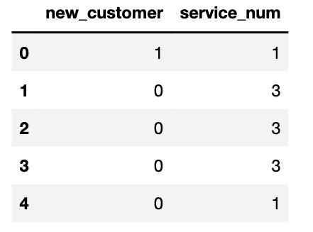
new_features = pd.DataFrame({'new_customer': new_customer, 'service_num': service_num})
new_features[:5]
features_test(new_features = new_features)
#49.44947409629822 s
#(0.8056795131845842,
# {'columntransformer__num': 'passthrough',
#  'logit_threshold__C': 0.1,
#  'logit_threshold__penalty': 'l2',
#  'logit_threshold__solver': 'newton-cg'},
#             accuracy_score  recall_score  precision_score  f1_score  \
# train_eval        0.807505      0.669104         0.554966  0.606714
# test_eval         0.797918      0.630573         0.540000  0.581783
#
#             roc_auc_score
# train_eval       0.758040
# test_eval        0.738246  )
The comparison results of different features are as follows:
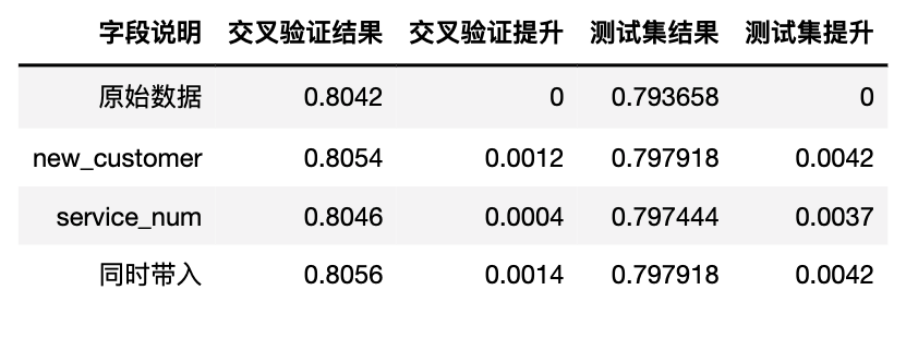
it can be found that the score of the new model on the verification set (0.805679) is slightly higher than the highest score of individual features, that is, new is brought in alone_ Customer score (0.8054766). Although the score on the test set is not higher than that brought in alone_ Customer, but as mentioned earlier, as long as the average score on the verification set increases, it indicates that the generalization ability of the model has been improved.
however, it should be known that in most cases, the superposition effect of features will not exceed the sum of the promotion effects of individual features. When there are too many new features, it may also lead to dimensional disaster, resulting in the decline of model effect. In addition, too much data will also lead to the increase of calculation time. Therefore, when many features are created, Features brought into modeling need to be carefully screened. More about feature filtering methods will be introduced at the end of this section.
2, Field creation based on data distribution law
if the field creation based on business experience is a feature derivation method based on general experience, the field creation method based on the current data distribution is a feature creation based on more in-depth analysis and more in line with the current actual situation. In most cases, feature derivation based on specific data conditions will be more effective. At the same time, the derived features can also be used as new business indicators to guide the actual business development.
- Effective features
of course, before creating and screening specific features, we can also further discuss "what features can better help the model modeling results". According to the previous analysis, we know that many times feature derivation is not to create more information, but to better present the existing information. Generally speaking, the greater the difference in the proportion of different categories corresponding to the features we create Then the feature is about helpful to help the model complete the training (for example, when the value of a created feature is 1, the corresponding data labels are all 1 or all 0).
Of course, with the in-depth analysis, we will further add some restrictions to this conclusion, such as distinguishing more samples and improving the effect compared with the original fields.
therefore, we need to start with those features that have a high degree of discrimination for the label (such as those with a particularly large loss rate or a particularly small loss rate), and in the process of analysis, we first use the stacking histogram previously used for analysis, and then give a more rigorous evaluation method of effective features.
1. Field exploration and feature derivation of demographic information
first, we analyze the user demographic attribute fields. In Part 1, we have visually analyzed the label value distribution of such fields, and the basic results are as follows:
- Analysis ideas
it is not difficult to find that in all three fields, the senior user field 'senior citizen' is a field with obvious differentiation. After simple statistical analysis, it is not difficult to find that nearly half of the elderly users have lost:
# Proportion of loss of elderly users
tcc[(tcc['SeniorCitizen'] == 1)]['Churn'].mean()
#0.4168126094570928
Such a small number of people have such a high loss rate, we might as well start with the elderly field for analysis. Of course, on the one hand, we can see that the products provided by the telecom operator are indeed not friendly to elderly users. At the same time, such a high loss rate of this field has also become a breakthrough for us to further explore the data. Generally speaking, fields with high response rate or numerical anomaly fields can become a breakthrough for further data exploration. Here, we focus on whether there is any other related field (i.e. user demographic information field) that has an important impact on the loss of elderly users. If so, the combination of the two fields can better mark whether users are lost. In other words, we want to start with the old field and create a new valid field by combining it with other associated fields.
- Numerical verification
there are three fields that belong to the same demographic information as the elderly field, 'dependencies',' Partner 'and' gender ', and each field has two value levels. We first extract the information of elderly users separately:
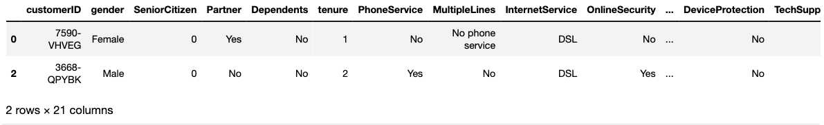
ts = tcc[tcc['SeniorCitizen'] == 1]
ts.head(2)
Then, similar to Part 1, observe the impact of different values of other different variables on whether users are lost by stacking histograms:
sns.set()
plt.figure(figsize=(16,12), dpi=200)

plt.subplot(221)
sns.countplot(x="Dependents",hue="Churn",data=ts,palette="Blues", dodge=False)
plt.xlabel("Dependents")
plt.title("Churn by Dependents")

plt.subplot(222)
sns.countplot(x="Partner",hue="Churn",data=ts,palette="Blues", dodge=False)
plt.xlabel("Partner")
plt.title("Churn by Partner")

plt.subplot(223)
sns.countplot(x="gender",hue="Churn",data=ts,palette="Blues", dodge=False)
plt.xlabel("gender")
plt.title("Churn by gender")
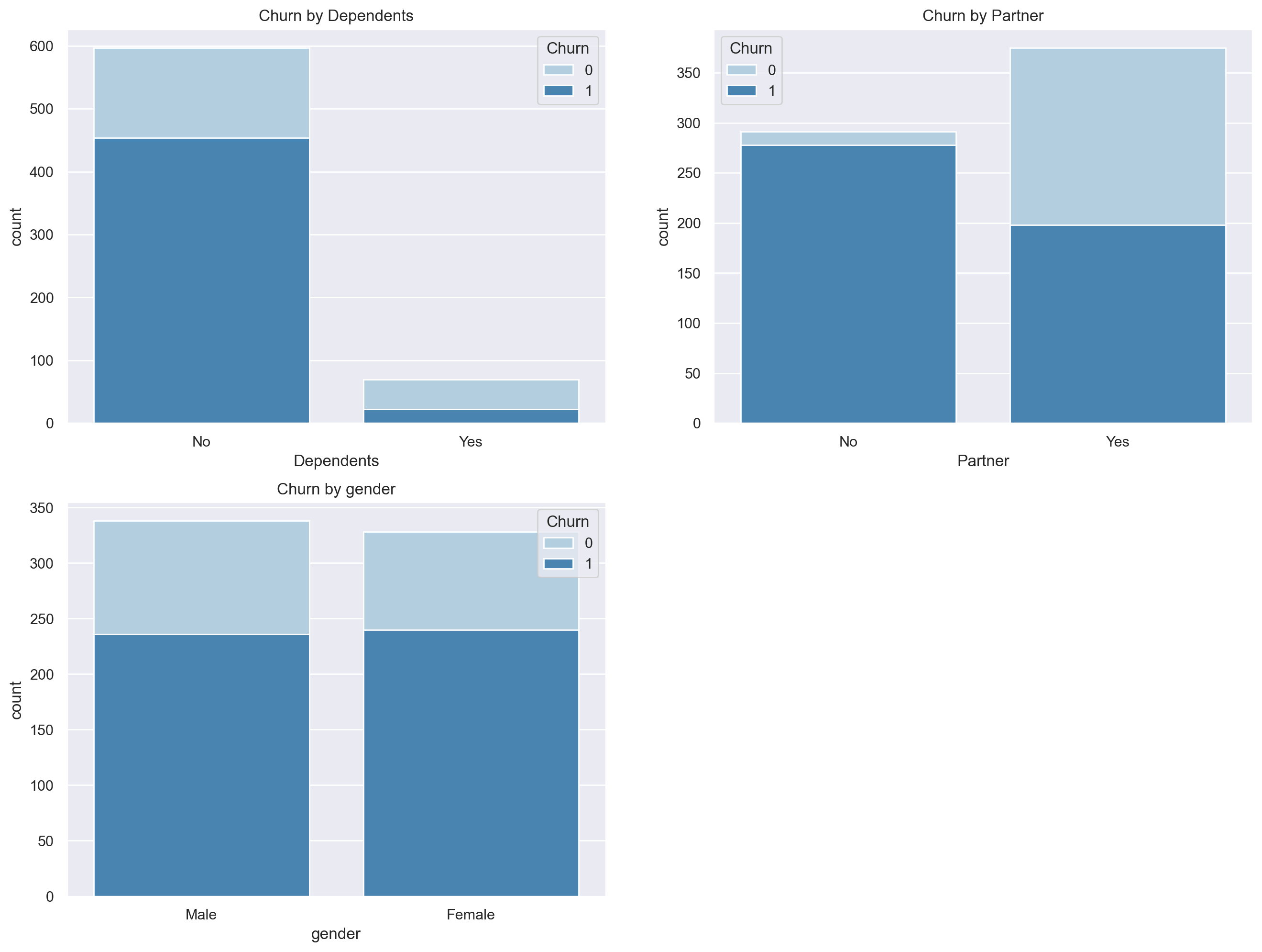
It can be found that the cross influence of gender field on the loss rate is not obvious for elderly users, while the cross influence of dependencies and partners field on the population of elderly users is more obvious, that is, the loss rate varies greatly in different values of the two fields. Of course, we focus on the cross influence combination results with high loss rate, That is, when the two fields are No, we can count the total number of people who meet the conditions and the turnover rate of the population in the following ways:
(ts[ts['Partner'] == 'No']['Churn'].mean(),
ts[ts['Partner'] == 'No']['Churn'].shape[0])
#(0.48857644991212656, 569)
(ts[ts['Dependents'] == 'No']['Churn'].mean(),
ts[ts['Dependents'] == 'No']['Churn'].shape[0])
#(0.4319695528068506, 1051)
Assuming that class A users are elderly users without partners and class B users are elderly users without economic independence, according to the above statistical results, we find that the loss rate of both types of users is higher than that of single elderly users, which shows that if we extract the division of these two groups of people can help us better identify the risk population, we can derive two different fields accordingly, That is, the elderly and no partner identification field (field A) and the elderly and uneconomic independent identification field (field B). At the same time, we also found that although the churn rate of class A users is 5% higher than that of class B users, the number of class A users is only half of that of class B users, which shows that although the division of class A population is effective, it does not necessarily have good universality, and the corresponding field A may not be as helpful to model modeling as field B.
- WOE calculation and IV value test
of course, which field will be more helpful for modeling? The most direct way is to bring it in separately for modeling, and then observe the final model output. However, if we need to compare the effect of two variables on model improvement without bringing it into modeling, there are also methods, which are the most common and widely verified and effective way to test the prediction ability of a variable, Is to calculate the value of IV(information value). The value of IV here has the same name as the value of IV in the decision tree, but the value of IV here is not based on C4 5, but a simple calculation process based on sample proportion. Its basic formula is as follows:
I
V
=
∑
i
=
1
N
I
V
i
=
∑
i
=
1
N
(
P
g
o
o
d
(
i
)
−
P
B
a
d
(
i
)
)
∗
W
O
E
i
=
∑
i
=
1
N
(
P
g
o
o
d
(
i
)
−
P
B
a
d
(
i
)
)
∗
l
n
P
G
o
o
d
(
i
)
P
B
a
d
(
i
)
IV = \sum^{N}_{i=1}IV_i=\sum^{N}_{i=1}(P_{good}^{(i)}-P_{Bad}^{(i)})*WOE_i= \sum^{N}_{i=1}(P_{good}^{(i)}-P_{Bad}^{(i)})*ln\frac{P_{Good}^{(i)}}{P_{Bad}^{(i)}}
IV=i=1∑NIVi=i=1∑N(Pgood(i)−PBad(i))∗WOEi=i=1∑N(Pgood(i)−PBad(i))∗lnPBad(i)PGood(i)
Firstly, the calculation result of IV value is the information value of a discrete variable in the binary classification problem, or the influence degree of the variable on the label value. The larger the IV value, the greater the influence of the field on the label value. Bringing it into the field can help the model predict more effectively. In the above calculation process, good/bad is only the different values of the label, which is equivalent to class 1 samples and Class 0 samples
i
i
i represents different values of a feature,
P
G
o
o
d
P_{Good}
PGood # and
P
B
a
d
P_{Bad}
PBad ^ is the proportion of class 1 and Class 0 samples in all class 1 / Class 0 samples calculated after grouping and summarizing under a certain value of the corresponding feature. Different values of each feature can be calculated into a group
I
V
i
IV_i
IVi, and eventually all within a feature
I
V
i
IV_i
The IV value of this feature can be calculated by summing IVi. Taking 'senior citizen' as an example, the total number of different types of users is:
tcc['Churn'].value_counts()
#0    5174
#1    1869
#Name: Churn, dtype: int64
When 'SeniorCitizen' is 1, the total number of different types of users in the divided sub dataset is:
tcc[tcc['SeniorCitizen'] == 1]['Churn'].value_counts()
#0    666
#1    476
#Name: Churn, dtype: int64
Based on this, we can calculate P G o o d ( 1 ) P^{(1)}_{Good} PGood(1) and P B a d ( 1 ) P^{(1)}_{Bad} PBad(1), now i = 1 i=1 i=1 indicates the calculation result of the sub dataset divided when the feature value is 1, while Good indicates class 1 samples and Bad indicates Class 0 samples:
PG1 = tcc[tcc['SeniorCitizen'] == 1]['Churn'].value_counts()[1] / tcc['Churn'].value_counts()[1]
PG1
#0.2546816479400749
That is, when the value of 'senior citizen' is 1, the proportion of the number of class 1 samples in the sub dataset to the number of class 1 samples in the total dataset. Of course, we can continue to calculate P B a d ( 1 ) P^{(1)}_{Bad} PBad(1):
PB1 = tcc[tcc['SeniorCitizen'] == 1]['Churn'].value_counts()[0] / tcc['Churn'].value_counts()[0]
PB1
#0.12872052570545034
That is, when 'SeniorCitizen' is 1, the proportion of the number of Class 0 samples in the sub dataset to the number of Class 0 samples in the total dataset. Based on this, we can further calculate I V 1 IV_1 IV1:
IV_1 = (PG1-PB1) * np.log(PG1/PB1)
IV_1
#0.08595218406217259
Similarly, we can continue to calculate I V 0 IV_0 IV0. At this time, i=0 indicates the calculation result of the sub dataset when the value of 'senior citizen' is 1:
PG0 = tcc[tcc['SeniorCitizen'] == 0]['Churn'].value_counts()[1] / tcc['Churn'].value_counts()[1]
PB0 = tcc[tcc['SeniorCitizen'] == 0]['Churn'].value_counts()[0] / tcc['Churn'].value_counts()[0]
IV_0 = (PG0-PB0) * np.log(PG0/PB0)
IV_0
#0.019668998791874313
The IV value of the final 'senior citizen' column is:
IV_0 + IV_1
#0.1056211828540469
Generally speaking, the larger the IV value, the more effective the feature is, and it is generally believed that the IV value has the following corresponding relationship with the feature effect:
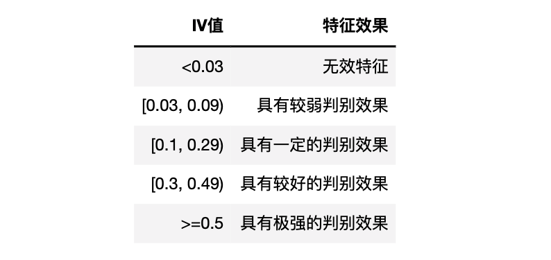
However, it should be noted that both the new field and the original features of the data can calculate the IV value, and the new field is generated by the original field. Therefore, the amount of information will overlap with the original field. If you need to judge whether the new field is useful through the IV value, you can't simply look at the IV value of the new field, but you need to compare the IV value of the new field with the original field, The value of the new field IV should be at least larger than the minimum value of the original field IV, and the new field is a valid field. Next, we will verify it.
More feature screening methods will be discussed later in this section
In addition to being a means of evaluating the importance of features, the calculation process of IV value and WOE is often used in continuous field boxes, especially in scorecard models.
- Function encapsulation
in the following content, we will frequently use IV value for feature importance evaluation. Here, we can first encapsulate the above calculation process into a function to facilitate subsequent calls:
def IV(new_features, DataFrame=tcc, target=target):
    count_result = DataFrame[target].value_counts().values

    def IV_cal(features_name, target, df_temp):
        IV_l = []
        for i in features_name:
            IV_temp_l = []
            for values in df_temp[i].unique():
                data_temp = df_temp[df_temp[i] == values][target]
                PB, PG = data_temp.value_counts().values / count_result
                IV_temp = (PG-PB) * np.log(PG/PB)
                IV_temp_l.append(IV_temp)
            IV_l.append(np.array(IV_temp_l).sum())
        return(IV_l)

    if type(new_features) == np.ndarray:
        features_name = ['new_features']
        new_features = pd.Series(new_features, name=features_name[0])
    elif type(new_features) == pd.Series:
        features_name = [new_features.name]
    else:
        features_name = new_features.columns

    df_temp = pd.concat([new_features, DataFrame], axis=1)
    df_temp = df_temp.loc[:, ~df_temp.columns.duplicated()]
    IV_l = IV_cal(features_name=features_name, target=target, df_temp=df_temp)

    res = pd.DataFrame(IV_l, columns=['IV'], index=features_name)
    return(res)

IV(tcc[['SeniorCitizen', 'Partner', 'Dependents']])

next, we use the above defined function to calculate the IV value of the identification field of class A (old and no partner) users and class B users (old and not economically independent):
custmer_A = (((tcc['SeniorCitizen'] == 1) & (tcc['Partner'] == 'No')) * 1).values
custmer_B = (((tcc['SeniorCitizen'] == 1) & (tcc['Dependents'] == 'No')) * 1).values
new_features = pd.DataFrame({'custmer_A':custmer_A, 'custmer_B':custmer_B})
IV(new_features)
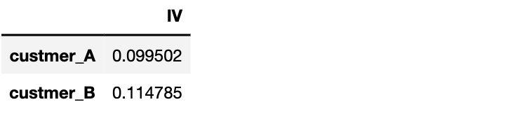
it can be found that the IV values of the two original fields used to create field A (0.105621 and 0.118729) are higher than that of field A (0.099502), while the IV value of field B (0.114785) is higher than that of the senior citizen field (0.105621). Therefore, we judge that field B is an available and effective field.
- Effect test
next, we will bring the above two fields into the model to test the actual effect:
features_test(new_features = custmer_A)
#44.55527067184448 s
#(0.8038539553752535,
# {'columntransformer__num': StandardScaler(),
#  'logit_threshold__C': 0.1,
#  'logit_threshold__penalty': 'l1',   #The advantage of collinearity between l1 regularization features is serious
#  'logit_threshold__solver': 'saga'},
#             accuracy_score  recall_score  precision_score  f1_score  \
# train_eval        0.806491      0.670401         0.544352  0.600837
# test_eval         0.792712      0.621212         0.521818  0.567194
#
#             roc_auc_score
# train_eval       0.757331
# test_eval        0.730957  )
features_test(new_features = custmer_B)
#42.324854135513306 s
#(0.8048681541582152,
# {'columntransformer__num': 'passthrough',
#  'logit_threshold__C': 0.30000000000000004,
#  'logit_threshold__penalty': 'l2',
#  'logit_threshold__solver': 'lbfgs'},
#             accuracy_score  recall_score  precision_score  f1_score  \
# train_eval        0.808519      0.668464         0.564064  0.611842
# test_eval         0.795078      0.618661         0.554545  0.584851
#
#             roc_auc_score
# train_eval       0.758911
# test_eval        0.733713  )
It can be found that compared with the original results (best_score=0.8042, the accuracy of the test set is 0.793658), field B can effectively improve the model effect, while field A is not helpful. Therefore, we can also see the effectiveness of IV value in helping feature screening.
At the same time, we can also find that if the characteristics are not properly brought in, it will have the opposite effect.
In addition, the above results are equivalent to indicating that the model effect can be improved by distinguishing the economically independent elderly. Further, we can build a new business index to know the development of the actual business, which is also an example of creating a business index through the algorithm.
- Summary of feature creation and screening process
of course, the above process of creating fields is a reusable process, and its basic process is as follows:
of course, since it is a method summary, we need to further try to verify the effectiveness of the method.
2. Contract period field exploration and feature derivation
next, we apply the above method to the analysis of user account fields. According to the data loss rate of Part 1, it is not difficult to find that the monthly payment rate is very high:
Next, let's start with the monthly paying users. Similarly, let's extract all monthly paying users separately:
cm = tcc[tcc['Contract'] == 'Month-to-month']
cm.head(2)
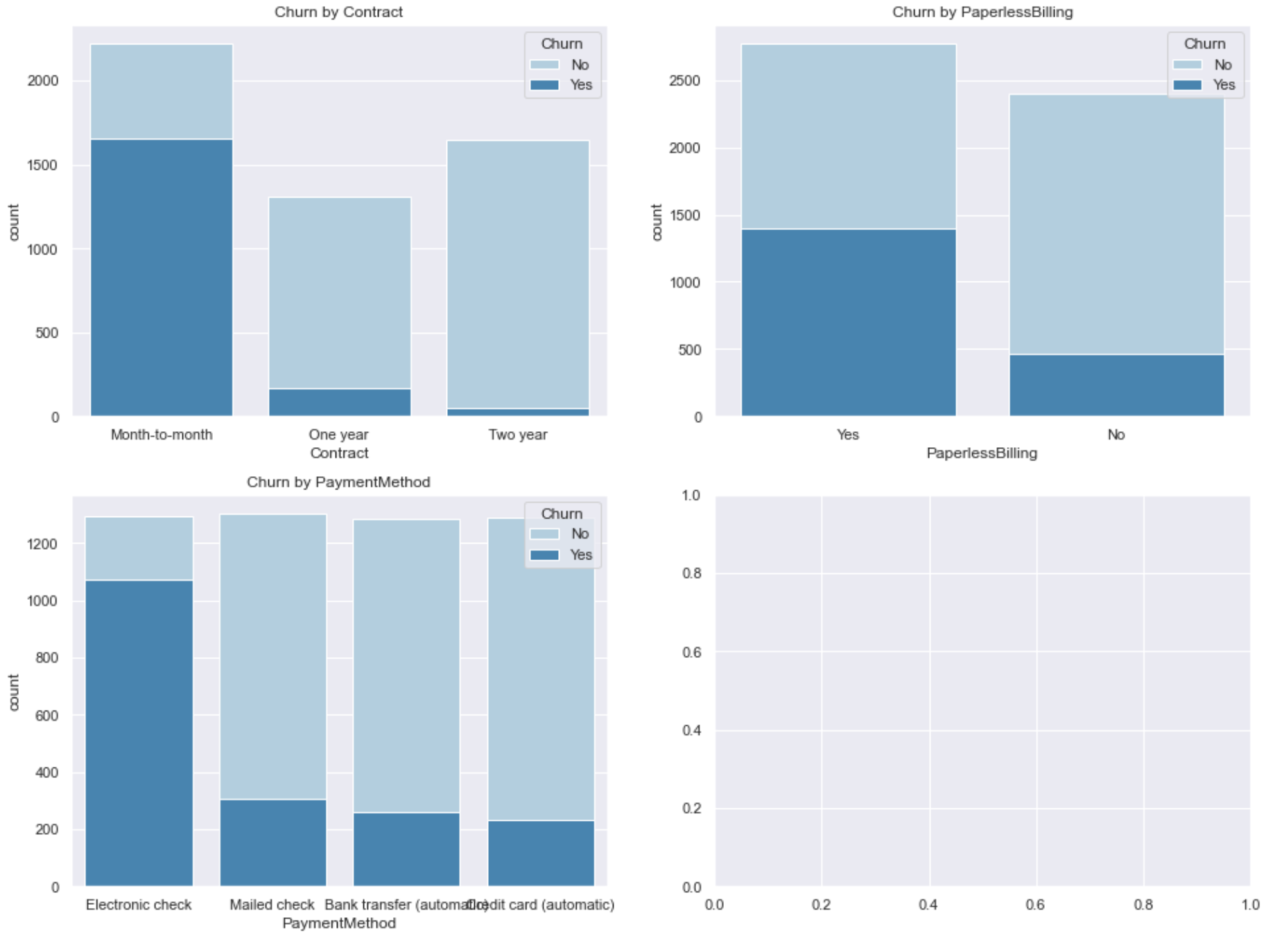
Then, similarly, we use the stacked histogram to analyze and observe the label distribution of other user account fields in different values among all monthly paying users:
sns.set()
plt.figure(figsize=(16,8), dpi=200)

plt.subplot(121)
sns.countplot(x="PaymentMethod",hue="Churn",data=cm,palette="Blues", dodge=False)
plt.xlabel("PaymentMethod")
plt.title("Churn by PaymentMethod")

plt.subplot(122)
sns.countplot(x="PaperlessBilling",hue="Churn",data=cm,palette="Blues", dodge=False)
plt.xlabel("PaperlessBilling")
plt.title("Churn by PaperlessBilling")
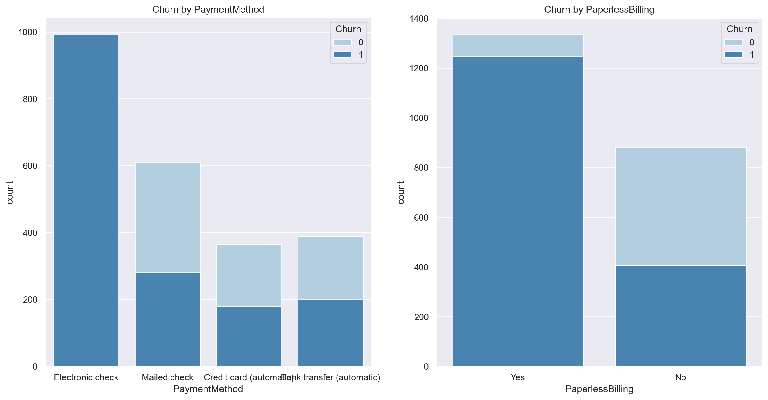
According to the graphic results, it is preliminarily judged that the turnover rate of users who pay monthly and pay through electronic channels is more than half. Of course, we need to further calculate:
(cm[cm['PaymentMethod'] == 'Electronic check']['Churn'].mean(),
cm[cm['PaymentMethod'] == 'Electronic check']['Churn'].shape[0])
#(0.5372972972972972, 1850)
(cm[cm['PaperlessBilling'] == 'Yes']['Churn'].mean(),
cm[cm['PaperlessBilling'] == 'Yes']['Churn'].shape[0])
#(0.48298530549110597, 2586)
A similar situation has emerged again. Among the users who pay monthly, the churn rate of users who pay electronically is high, but the number is small, while there are more users who pay paperless billing (electronic contract), but the churn rate is relatively low. Based on the above results, we can create two composite fields, namely, monthly payment and electronic channel payment account (a) and monthly payment and no paper contract account (B). These two fields are the fields that we judge are most likely to improve the model effect according to the above visualization results (the difference between the label distribution and the original label distribution is the largest), The creation process of two types of account identification fields is as follows:
account_A = (((tcc['Contract'] == 'Month-to-month') & (tcc['PaymentMethod'] == 'Electronic check')) * 1).values
account_B = (((tcc['Contract'] == 'Month-to-month') & (tcc['PaperlessBilling'] == 'Yes')) * 1).values
Next, verify the IV values of the two fields and the original field IV values involved in creating the new field:
# Original field IV value
IV(tcc[['Contract', 'PaymentMethod', 'PaperlessBilling']])

# New field IV value
new_features = pd.DataFrame({'account_A':account_A, 'account_B':account_B})
IV(new_features)
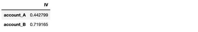
It can be found that the IV value of field A is lower than the minimum value of the original field participating in the creation of field A, while the IV value of field B is higher than the minimum value of the original field participating in the creation. Therefore, we judge that field B will be more effective than field A. Next, we bring the two fields into the model for inspection. The results are as follows:
features_test(new_features = account_A)
#44.69138741493225 s
#(0.8040567951318458,
# {'columntransformer__num': StandardScaler(),
#  'logit_threshold__C': 0.1,
#  'logit_threshold__penalty': 'l1',
#  'logit_threshold__solver': 'saga'},
#             accuracy_score  recall_score  precision_score  f1_score  \
# train_eval        0.806491      0.670401         0.544352  0.600837
# test_eval         0.792712      0.621212         0.521818  0.567194
#
#             roc_auc_score
# train_eval       0.757331
# test_eval        0.730957  )
features_test(new_features = account_B)
#41.55269169807434 s
#(0.804868154158215,
# {'columntransformer__num': 'passthrough',
#  'logit_threshold__C': 0.1,
#  'logit_threshold__penalty': 'l2',
#  'logit_threshold__solver': 'lbfgs'},
#             accuracy_score  recall_score  precision_score  f1_score  \
# train_eval        0.808316      0.667563         0.564822  0.611910
# test_eval         0.795551      0.620408         0.552727  0.584615
#
#             roc_auc_score
# train_eval       0.758532
# test_eval        0.734418  )
The modeling result is consistent with the expectation, indicating that the method is effective. On this basis, you can further try the combination and screening of other fields.
generally speaking, compared with the field creation process based on business experience, the field creation process based on data exploration is more "traceable", and some methods involved in the above process, including cross derivation discrete features and IV value screening features, will also be helpful for subsequent batch field creation.