Early Stopping

Brief Introduction

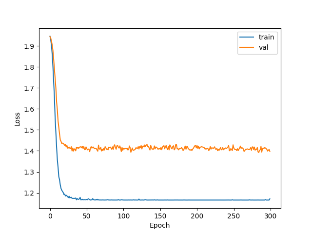
When we train deep learning neural networks, we usually hope to obtain the best generalization performance. However, all standard deep learning neural network structures such as MLP are easy to over fit: when the error rate of the network in the training set is getting lower and lower, in fact, at a certain moment, its performance in the test set has begun to deteriorate.

PS: in this figure, due to the small disturbance of the loss of the verification set, the "U-shape" of the verification set is not very obvious.

How to slove overfitting

1. Reduce the dimension of parameter space.
2. Reduce the effective scale of each dimension.
Methods to reduce the number of parameters include green constructive learning, pruning and weight sharing. The main methods to reduce the effective scale of each parameter dimension are regularization, such as weight decay and early stopping.

Early stopping

Brief Introduction

During training, calculate the performance of the model in the verification set. When the performance of the model in the verification set begins to decline, stop training.

Specific steps

Step 1: divide the training set into training set and verification set
Step 2: the training will be conducted only on the training set, and the error of the model on the verification set will be calculated for each cycle T, for example, one cycle in every 15 epoch (mini batch) training, and the optimal model parameters under the current situation will be saved.
step3: stop training when p times of bad verification set performance is observed (P can be understood as patience value and tolerance).
Step 4: use the parameters in the last iteration result as the final parameters of the model.

Codes

The following is an example to use early stopping, using a simple three-tier GCN as an example.

Pytorch = 1.7.1 ， Python = 3.6 ，torch-geomatric = 1.7.1,  CUDA = 10.1

import random
import torch
import torch.nn.functional as F
from torch_geometric.nn import GCNConv
from torch_geometric.datasets import Planetoid
import matplotlib.pyplot as plt

# Define the network used, layer 3 GCN
class GCN_NET3(torch.nn.Module):
    '''
    three-layers GCN
    two-layers GCN has a better performance
    '''
    def __init__(self, num_features, hidden_size1, hidden_size2, classes):
        '''
        :param num_features: each node has a [1,D] feature vector
        :param hidden_size1: the size of the first hidden layer
        :param hidden_size2: the size of the second hidden layer
        :param classes: the number of the classes 
        '''
        super(GCN_NET3, self).__init__()
        self.conv1 = GCNConv(num_features, hidden_size1)
        self.relu = torch.nn.ReLU()
        self.dropout = torch.nn.Dropout(p=0.5)  # use dropout to over ove-fitting
        self.conv2 = GCNConv(hidden_size1, hidden_size2)
        self.conv3 = GCNConv(hidden_size2, classes)
        self.softmax = torch.nn.Softmax(dim=1) # each raw

    def forward(self, Graph):
        x, edge_index = Graph.x, Graph.edge_index
        out = self.conv1(x, edge_index)
        out = self.relu(out)
        out = self.dropout(out)
        out = self.conv2(out, edge_index)
        out = self.relu(out)
        out = self.dropout(out)
        out = self.conv3(out, edge_index)
        out = self.softmax(out)
        return out

def setup_seed(seed):
    torch.manual_seed(seed)
    torch.cuda.manual_seed_all(seed)
    random.seed(seed)


dataset = Planetoid(root='./', name='Cora')  # if root='./', Planetoid will use local dataset
device = torch.device('cuda' if torch.cuda.is_available() else 'cpu')  # use cpu or gpu
model = GCN_NET3(dataset.num_node_features, 128, 64, dataset.num_classes).to(device)
data = dataset[0].to(device)
optimizer = torch.optim.Adam(model.parameters(), lr=0.005)  # define optimizer

# define some parameters
eval_T = 5  # evaluate period
P = 3  # patience
i = 0  # record the frequency f bad performance of validation
max_epoch = 300
setup_seed(seed=20)  # set up random seed
temp_val_loss = 99999  # initialize val loss
L = []  # store loss of training
L_val = []  # store loss of val

# training process
model.train()
for epoch in range(max_epoch):
    optimizer.zero_grad()
    out = model(data)
    loss = F.cross_entropy(out[data.train_mask], data.y[data.train_mask])
    _, val_pred = model(data).max(dim=1)
    loss_val = F.cross_entropy(out[data.val_mask], data.y[data.val_mask])

    # early stopping
    if (epoch % eval_T) == 0:
        if (temp_val_loss > loss_val):
            temp_val_loss = loss_val
            torch.save(model.state_dict(), "GCN_NET3.pth")  # save th current best
            i = 0  # reset i
        else:
            i = i + 1
    if i > P:
        print("Early Stopping! Epoch : ", epoch,)
        break

    L_val.append(loss_val)
    val_corrent = val_pred[data.val_mask].eq(data.y[data.val_mask]).sum().item()
    val_acc = val_corrent / data.val_mask.sum()
    print('Epoch: {}  loss : {:.4f}  val_loss: {:.4f}  val_acc: {:.4f}'.format(epoch, loss.item(),
                                                                               loss_val.item(), val_acc.item()))
    L.append(loss.item())
    loss.backward()
    optimizer.step()

# test
model.load_state_dict(torch.load("GCN_NET3.pth"))   # load parameters of the model
model.eval()
_, pred = model(data).max(dim=1)
corrent = pred[data.test_mask].eq(data.y[data.test_mask]).sum().item()
acc = corrent / data.test_mask.sum()
print("test accuracy is {:.4f}".format(acc.item()))

# plot the curve of loss

n = [i for i in range(len(L))]
plt.plot(n, L, label='train')
plt.plot(n, L_val, label='val')
plt.legend()  # show the labels
plt.xlabel('Epoch')
plt.ylabel('Loss')
plt.show()

Result

Output result:
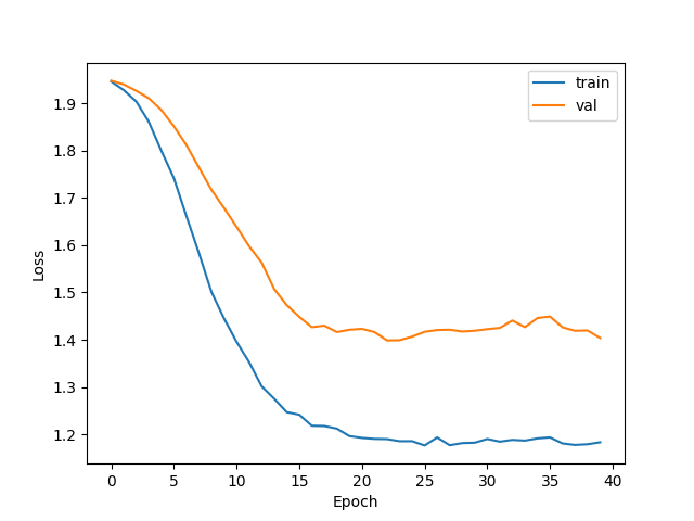
Early Stopping!  Epoch :  28
test accuracy is 0.8030

The test accuracy has been significantly improved. When Early stopping is not used, the test accuracy is about 76%; Now it is about 78%, up to 80.3%

Disadvantages

1. If the training ends too early, the cost function will be large, and the situation to be considered is more complex. At the same time, it is possible to obtain a local optimal solution or suboptimal solution.
2. The calculation cost will be increased during training. In practice, the evaluation cost can be reduced by parallel early stopping on a CPU or GPU independent of the main training process, or less frequent evaluation and verification sets.
3. You need to save the best training copy when you need a certain storage space.

Reference

1. Deep learning - Ian goodflow
2.GCN, GraphSAGE, and GAT are implemented using Python geometry