Introduction 
In this experiment, we will implement the principal component analysis method and use it to obtain the low dimensional representation of face image.
The data sets used in this experiment include:
ex4data1.mat -2D simulation dataset
ex4data2.mat -LFW face dataset
The scoring criteria are as follows:
Key point 1: realize PCA algorithm ------------ (20 points)
Key point 2: dimension reduction simulation data ------------ (20 points)
Key point 3: reconstruct simulation data ------------ (20 points)
Key point 4: dimensionality reduction of face data ------------ (20 points)
Key point 5: reconstruct face data ------------ (20 points)
# Import the required library files
import os
import numpy as np
import pandas as pd
import matplotlib.pyplot as plt
import matplotlib as mpl
import seaborn as sb
from scipy.io import loadmat
import scipy

%matplotlib inline
1. Realize principal component analysis
In this part of the experiment, the principal component analysis algorithm will be implemented. The algorithm steps are as follows:
Step 1: standardize all samples so that the mean value of the samples is 0 and the standard deviation is 1
Step 2: calculate the covariance matrix of the sample: X X T \mathbf{X}\mathbf{X}^T XXT
Step 3: pair covariance matrix X X T \mathbf{X}\mathbf{X}^T XXT performs eigenvalue decomposition (or singular value decomposition)
Step 4: take the largest d d Eigenvector corresponding to d eigenvalues w 1 , ⋯ , w d \mathbf{w}_1,\cdots,\mathbf{w}_{d} w1,⋯,wd
Output: projection matrix W = [ w 1 , ⋯ , w d ] \mathbf{W}=[\mathbf{w}_1,\cdots,\mathbf{w}_{d}] W=[w1,⋯,wd]
# ======================Fill in the code here=======================
def PCA(X,d):
    """
    input
    ----------
    X : Size (D, m)Matrix of, page i Listed as No i Samples, D Is the dimension of the sample, m Is the number of samples.

    d:  Expected dimension

    output
    -------
    W : Size (D, d)Projection matrix, section i The second column of the covariance matrix i An eigenvector.
    """

    X=[(x-np.mean(x))/np.std(x,axis=0,ddof=1) for x in X]
    matrix=np.cov(X[0],X[1])
    X=np.array(X)
    Z=np.matmul(X,X.T)
    U,S,V=np.linalg.svd(Z)
    W=U[:,:d]
    return W
# =============================================================
If the above function pca is completed, the following code can be used for testing. If the result is [- 0.707107, - 0.707107], the calculation passes.
# Load the dataset into the variable X
data = loadmat(os.path.join('ex4data1.mat'))
X = data['X']

#  Run PCA
W= PCA(X.T,2)


print('First eigenvector: W[:, 0] = [{:.6f}, {:.6f}]'.format(W[0, 0], W[1, 0]))
First eigenvector: W[:, 0] = [-0.707107, -0.707107]
2 apply PCA to simulation data
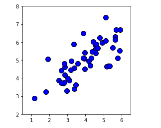
In this part of the experiment, the realized PCA algorithm is applied to data set 1. The sample dimension of the data set is 2. Therefore, after dimensionality reduction, the results before and after dimensionality reduction can be observed visually.
#  Visualizing raw data sets
plt.plot(X[:, 0], X[:, 1], 'bo', ms=10, mec='k', mew=1)
plt.axis([0.5, 6.5, 2, 8])
plt.gca().set_aspect('equal')
plt.grid(False)
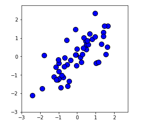
#  Visualization of standardized data sets
mu = np.mean(X,axis=0)
sigma = np.std(X,axis=0)
X_norm = (X - mu)/sigma
plt.plot(X_norm[:, 0], X_norm[:, 1], 'bo', ms=10, mec='k', mew=1)
plt.axis([-3, 2.75, -3, 2.75])
plt.gca().set_aspect('equal')
plt.grid(False)
2.1 dimensionality reduction using PCA
The above PCA code can reduce the simulation data to one dimension.
# ======================Fill in the code here=======================
def ProjectData(X, W):
    """
    input
    ----------
    X : Size (D, m)Matrix of, page i Listed as No i Samples, D Is the dimension of the sample, m Is the number of samples.
    W : Size (D, d)Projection matrix, section i The second column of the covariance matrix i An eigenvector.

    output
    -------
    Z : Size (d, m)Matrix of, page i Listed as No i Data after dimensionality reduction.
    """
    X=[(x-np.mean(x))/np.std(x,axis=0,ddof=1) for x in X]
    Z=np.matmul(W.T,X)


    return Z
# =============================================================
If the above function ProjectData is completed, the following code can be used for testing. If the result is 1.481274, the calculation passes.
#  Reduce data to one dimension
W = PCA(X.T,1)
Z = ProjectData(X.T, W)
print('Data after dimension reduction of the first sample: {:.6f}'.format(Z[0, 0]))
Data after dimension reduction of the first sample: 1.481274
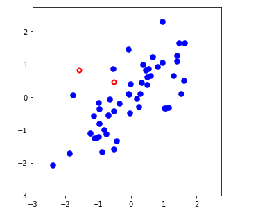
2.2 reconstruct the original data through the reduced dimension data
Using the reduced dimension data matrix Z \mathbf{Z} Z. The original data can be approximately reconstructed.
# ======================Fill in the code here=======================
def RecoverData(Z, W):
    """
    input
    ----------
    Z : Size (d, m)Matrix of, page i Listed as No i Data after dimensionality reduction.
    W : Size (D, d)Projection matrix, section i The second column of the covariance matrix i An eigenvector.

    output
    -------
    X_rec : Size (D, m)Matrix of, page i Listed as No i A reconstructed data.
    """
    W=np.matrix(W)
    X_rec=np.dot(W.T.I,Z)


    return X_rec
# =============================================================
If the above function RecoverData is completed, the following code can be used for testing. If the result is [- 1.047419, - 1.047419], the calculation passes.
#  Reconstruct original data
X_rec = RecoverData(Z, W).T

# print('first reconstructed data: {:. 6f}'.format(X_rec[:, 0]))
print('The first reconstructed data: X_rec[0, :] = [{:.6f}, {:.6f}]'.format(X_rec[0, 0], X_rec[0, 1]))
First reconstructed data: X_rec[0, :] = [-1.047419, -1.047419]
mu = np.mean(X,axis=0)
sigma = np.std(X,axis=0, ddof=1)
X_norm = (X - mu)/sigma

#  Plot the normalized dataset (returned from featureNormalize)
fig, ax = plt.subplots(figsize=(5, 5))
ax.plot(X_norm[:, 0], X_norm[:, 1], 'bo', ms=8, mec='b', mew=0.5)
ax.set_aspect('equal')
ax.grid(False)
plt.axis([-3, 2.75, -3, 2.75])

# Draw lines connecting the projected points to the original points
ax.plot(X_rec[:, 0], X_rec[:, 1], 'ro', mec='r', mew=2, mfc='none')
for xnorm, xrec in zip(X_norm, X_rec):
    ax.plot([xnorm[0], xrec[0]], [xnorm[1], xrec[1]], '--k', lw=1)
3 apply PCA to face reconstruction
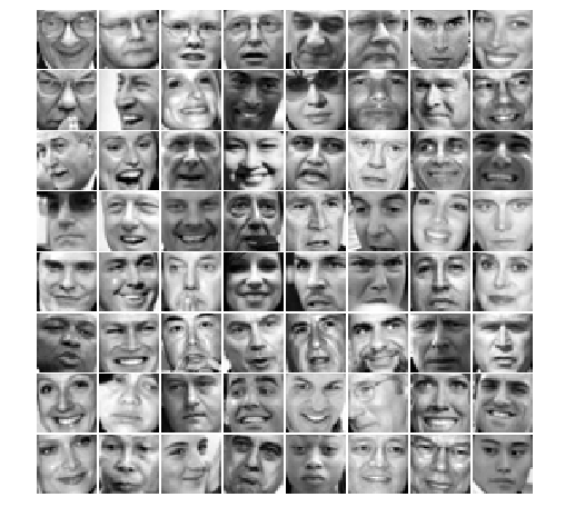
In this part of the experiment, the implemented PCA algorithm is applied to dataset 2, which is a subset of LFW face data set.
#  Load Face dataset
data = loadmat(os.path.join( 'ex4data2.mat'))
X = data['X']
#Define functions to display face images
def displayData(X, example_width=None, figsize=(8, 8)):

    """
    input
    ----------
    X : Size (m, D)Matrix of, page i Listed as No i Samples, D Is the dimension of the sample, m Is the number of samples.
    """

    # Compute rows, cols
    if X.ndim == 2:
        m, n = X.shape
    elif X.ndim == 1:
        n = X.size
        m = 1
        X = X[None]  # Promote to a 2 dimensional array
    else:
        raise IndexError('Input X should be 1 or 2 dimensional.')

    example_width = example_width or int(np.round(np.sqrt(n)))
    example_height = int(n / example_width)

    # Compute number of items to display
    display_rows = int(np.floor(np.sqrt(m)))
    display_cols = int(np.ceil(m / display_rows))

    fig, ax_array = plt.subplots(display_rows, display_cols, figsize=figsize)
    fig.subplots_adjust(wspace=0.025, hspace=0.025)

    ax_array = [ax_array] if m == 1 else ax_array.ravel()

    for i, ax in enumerate(ax_array):
        ax.imshow(X[i].reshape(example_height, example_width, order='F'), cmap='gray')
        ax.axis('off')
 #  Display the first 100 faces in the dataset
displayData(X[:64, :], figsize=(8, 8))
3.1 dimensionality reduction of face image using PCA
# ======================Fill in the code here=======================
W1=PCA(X.T,64)
print(W1[:36])
Z1=ProjectData(X.T,W1)


# =============================================================
[[-0.01425307 -0.03606596 -0.04561884 ...  0.0061877   0.02367001
   0.05076207]
 [-0.01474233 -0.03809858 -0.04756249 ...  0.00101133  0.01959809
   0.05250727]
 [-0.01501482 -0.03988747 -0.05082085 ... -0.00338655  0.00776122
   0.05543446]
 ...
 [-0.01711169 -0.04114578 -0.04517263 ...  0.0064823   0.0409063
   0.02625426]
 [-0.01721429 -0.04300162 -0.04873793 ...  0.00549935  0.02761684
   0.03023218]
 [-0.01742302 -0.04464136 -0.05105597 ...  0.01009193  0.00885712
   0.03474425]]
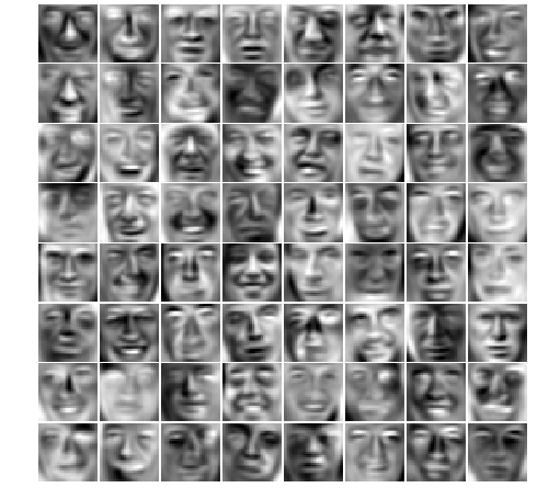
3.2 reconstruction of original face data by principal component
# ======================Fill in the code here=======================
X1_rec=RecoverData(Z1,W1).T

displayData(X1_rec[:64,:],figsize=(8,8))
# =============================================================
