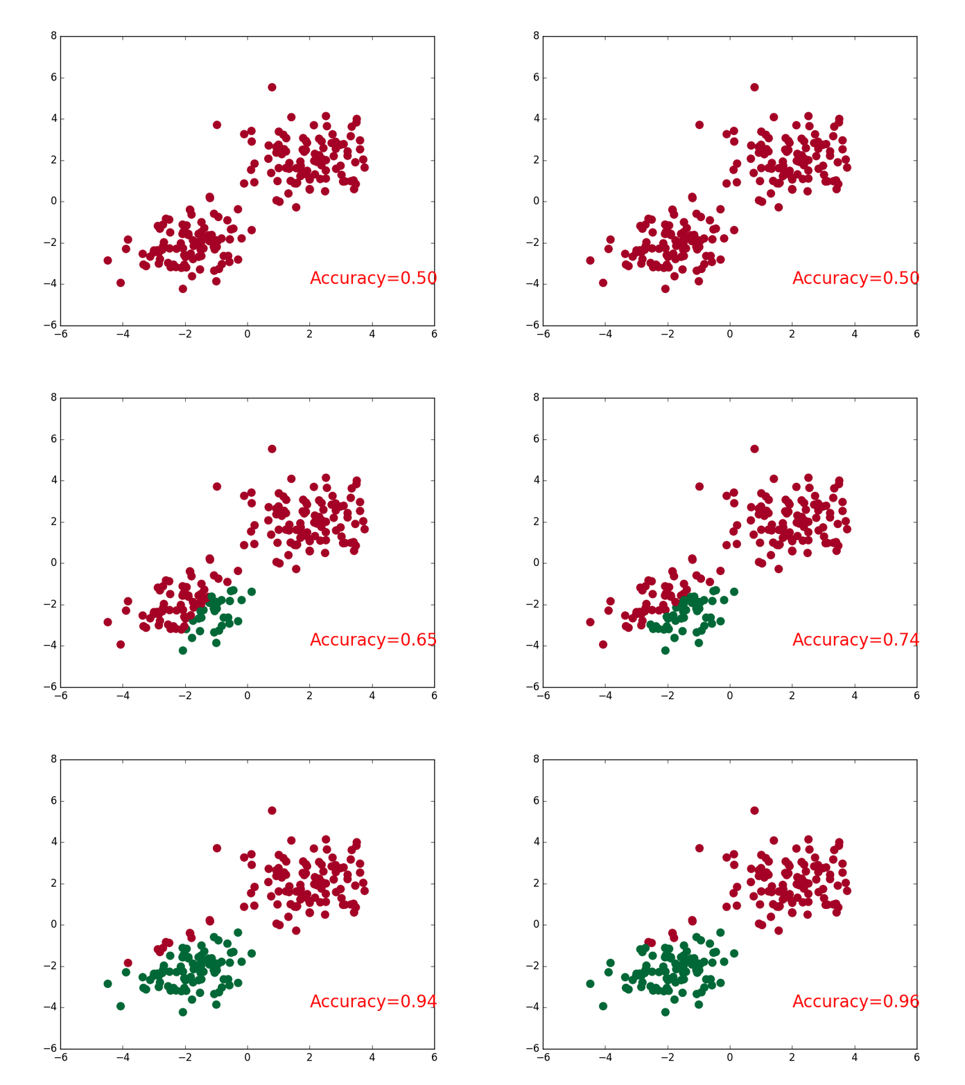
I. Description:

Take a simple example to see how neural networks are classified.

Two, steps

1. Create data

import torch
import matplotlib.pyplot as plt
import torch.functional as func
from torch.autograd import Variable
import torch.nn

#There are two groups of data, one belongs to Category 1 and the other belongs to Category 0.

#Create data
n_data=torch.ones(100,2)
data1=torch.normal(2*n_data,1)   #The x and y coordinates of a set of data are included in data1.
label1=torch.zeros(100)           #Data 1 The labels for this stack of data are all 0.
data2=torch.normal(-2*n_data,1)  #Another pile of data
label2=torch.ones(100)            #Data 2 This stack of data has labels of 1
#Data data and the corresponding classification labels for each data
data=torch.cat((data1,data2),0).type(torch.FloatTensor)   #All data. cat: merging data sets
labels=torch.cat((label1,label2),0).type(torch.LongTensor)     #All labels

Note:

• torch.normal() function

torch.normal(measn,std,out=None) returns a tensor containing random numbers extracted from the discrete normal distribution of the given parameter means,std.
Mean: A tensor that contains the mean of the normal distribution associated with each output element.
std: a tensor that contains the standard deviation of the positive distribution of each output element. The standard deviation must be a positive number.
The shape of mean and standard deviation may not match, but the number of elements in each tensor must be the same.

import torch

# method1, mean and standard deviation are matrices
means=2.0*torch.ones(3,2)
std=torch.ones(3,2)
tensor1=torch.normal(means,std)
print('tensor1:\n',tensor1)

# Method 2, Sample Sharing Mean
tensor2=torch.normal(1,torch.arange(1.0,4.0))
print('tensor2:\n',tensor2)

# Method 3, Sample Sharing Standard Deviation
tensor3=torch.normal(torch.arange(1,0,-0.2),0.2)
print('tensor3:\n',tensor3)

Operation results:

tensor1:
 tensor([[ 2.2218,  1.7356],
        [ 2.3562,  1.8443],
        [-0.3917,  1.4340]])
tensor2:
 tensor([0.1562, 2.5264, 0.4343])
tensor3:
 tensor([1.2139, 0.6693, 0.7391, 0.5015, 0.4305])

• torch.cat() function: merging two matrices

import torch

tensor1=torch.rand((3,2))
tensor2=torch.normal(torch.ones(3,2),0.4)

tensor_cat0=torch.cat((tensor1,tensor2),0)
tensor_cat1=torch.cat((tensor1,tensor2),1)
print(
    'tensor_cat0:\n',tensor_cat0,
    '\ntensor_cat1:\n',tensor_cat1
)

Operation results:

tensor_cat0:
 tensor([[0.1172, 0.8874],
        [0.5329, 0.3272],
        [0.8525, 0.9647],
        [1.4242, 0.8938],
        [0.6884, 1.8814],
        [0.9747, 0.9873]]) 
tensor_cat1:
 tensor([[0.1172, 0.8874, 1.4242, 0.8938],
        [0.5329, 0.3272, 0.6884, 1.8814],
        [0.8525, 0.9647, 0.9747, 0.9873]])

2. Building Neural Networks

#Building Neural Network
x=Variable(data)
y=Variable(labels)
class Net(torch.nn.Module):
    def __init__(self,n_feature,n_hidden,n_output):
        super(Net, self).__init__()
        self.hidden=torch.nn.Linear(n_feature,n_hidden)
        self.output=torch.nn.Linear(n_hidden,n_output)

    def forward(self,x):
        a_i=torch.relu(self.hidden(x))
        h_x=self.output(a_i)
        return h_x

Note:

• torch.nn.Linear()

class torch.nn.linear(in_features,out_features,bias=True) performs a linear transformation of the incoming data: y=ax+b
 in_features: the size of input data; out_features: the size of output data
 Bias: The default is True, indicating that the layer will learn additional bias

 

import torch.nn
from torch.autograd import Variable

h_x=torch.nn.Linear(in_features=2,out_features=4)
in_features=Variable(torch.rand(3,2))    #Random Generation of 3*2 Random Number Matrix in [0,1] Interval
out_features=h_x(in_features)
print(out_features)
print(out_features.size())       #out_features.size()=(3*2)*(2*4)=3*4

Operation results:

tensor([[-0.5179, -0.4531,  0.2644, -0.1680],
        [-1.1484, -0.8473,  0.2247, -0.1441],
        [-0.7792, -0.6470,  0.2994, -0.1619]], grad_fn=<AddmmBackward>)
torch.Size([3, 4])

3. Training network and visualization

#Training network
net=Net(2,10,2)    #Input is two features, coordinates x and y; output two classifications 0 and 1
optomizer=torch.optim.SGD(net.parameters(),lr=0.01)
loss_func=torch.nn.CrossEntropyLoss()  #Cross Entropy Loss Function

for i in range(100):
    out=net.forward(x)
    loss=loss_func(out,y)

    optomizer.zero_grad()
    loss.backward()
    optomizer.step()

    #visualization
    if i%2==0:
        plt.cla()                        #Clear the original image
        prediction=torch.max(out,1)[1]   #torch.max(out,1) returns the value and index of the maximum value of each row. prediction represents the index of all maximum values, i.e. classification
        pred_y=prediction.data.numpy()
        target_y=y.data.numpy()
        plt.scatter(x.data.numpy()[:,0],x.data.numpy()[:,1],c=pred_y,s=100,cmap='RdYlGn') #c: Color or color sequence, s: point size
        accuracy=float((pred_y==target_y).astype(int).sum())/float(target_y.size)  #astype() type conversion
        plt.text(1.5,-4,'Accuracy=%.2f'%accuracy,fontdict={'size':15,'color':'purple'})
        plt.pause(0.1)

plt.show()