preface

The actual combat series of this project is mainly based on the tutorials on the network. It mainly refers to the ideas and specific implementation codes in learning machine learning with Digo. However, the version used in the book should be python2. Some codes also have problems, some key steps are omitted, and some are syntax problems, In short, it can not run all the way directly. Here we have sorted out the code and data set that can run (the link is easy to hang, please chat privately).

Series navigation

• Credit card fraud based on logistic regression
• Random forest temperature prediction
• News classification based on Bayesian
• Music recommendation platform based on recommendation system
• ...

Import data

import pandas as pd
import matplotlib.pyplot as plt
import numpy as np
%matplotlib inline
data = pd.read_csv("creditcard.csv")
data.head()

	Time	V1	V2	V3	V4	V5	V6	V7	V8	V9	...	V21	V22	V23	V24	V25	V26	V27	V28	Amount	Class
0	0.0	-1.359807	-0.072781	2.536347	1.378155	-0.338321	0.462388	0.239599	0.098698	0.363787	...	-0.018307	0.277838	-0.110474	0.066928	0.128539	-0.189115	0.133558	-0.021053	149.62	0
1	0.0	1.191857	0.266151	0.166480	0.448154	0.060018	-0.082361	-0.078803	0.085102	-0.255425	...	-0.225775	-0.638672	0.101288	-0.339846	0.167170	0.125895	-0.008983	0.014724	2.69	0
2	1.0	-1.358354	-1.340163	1.773209	0.379780	-0.503198	1.800499	0.791461	0.247676	-1.514654	...	0.247998	0.771679	0.909412	-0.689281	-0.327642	-0.139097	-0.055353	-0.059752	378.66	0
3	1.0	-0.966272	-0.185226	1.792993	-0.863291	-0.010309	1.247203	0.237609	0.377436	-1.387024	...	-0.108300	0.005274	-0.190321	-1.175575	0.647376	-0.221929	0.062723	0.061458	123.50	0
4	2.0	-1.158233	0.877737	1.548718	0.403034	-0.407193	0.095921	0.592941	-0.270533	0.817739	...	-0.009431	0.798278	-0.137458	0.141267	-0.206010	0.502292	0.219422	0.215153	69.99	0

5 rows × 31 columns

Get the data

1. Consider the ratio of abnormal value to normal value and whether the sample distribution is uniform

count_classes = pd.value_counts(data['Class'], sort=True).sort_index()
count_classes.plot(kind='bar')
plt.title("class analysis")
plt.xlabel("classes")
plt.ylabel("frequency")

Text(0, 0.5, 'frequency')

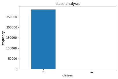
1. It is observed that there are too few outliers in the data set, and our model should pay attention to the outliers

Data preprocessing

Solve the problem of data label imbalance

1. Down sampling: normal samples are as few as abnormal samples
2. Oversampling, falsifying abnormal data to make its data volume reach the normal level
   The two cases need to be compared

Feature standardization

The units of each column are different and the degree of change is different. The data needs to be improved. After data processing, the value of each feature is floating in a small range
Z = X − X m e a n s t d ( X ) Z = \frac{X-X_{mean}}{std(X)} Z=std(X)X−Xmean​​

from sklearn.preprocessing import StandardScaler
data['normAmount'] = StandardScaler().fit_transform(data['Amount'].values.reshape(-1,1))
data = data.drop(['Time','Amount'],axis=1)
data.head()

	V1	V2	V3	V4	V5	V6	V7	V8	V9	V10	...	V21	V22	V23	V24	V25	V26	V27	V28	Class	normAmount
0	-1.359807	-0.072781	2.536347	1.378155	-0.338321	0.462388	0.239599	0.098698	0.363787	0.090794	...	-0.018307	0.277838	-0.110474	0.066928	0.128539	-0.189115	0.133558	-0.021053	0	0.244964
1	1.191857	0.266151	0.166480	0.448154	0.060018	-0.082361	-0.078803	0.085102	-0.255425	-0.166974	...	-0.225775	-0.638672	0.101288	-0.339846	0.167170	0.125895	-0.008983	0.014724	0	-0.342475
2	-1.358354	-1.340163	1.773209	0.379780	-0.503198	1.800499	0.791461	0.247676	-1.514654	0.207643	...	0.247998	0.771679	0.909412	-0.689281	-0.327642	-0.139097	-0.055353	-0.059752	0	1.160686
3	-0.966272	-0.185226	1.792993	-0.863291	-0.010309	1.247203	0.237609	0.377436	-1.387024	-0.054952	...	-0.108300	0.005274	-0.190321	-1.175575	0.647376	-0.221929	0.062723	0.061458	0	0.140534
4	-1.158233	0.877737	1.548718	0.403034	-0.407193	0.095921	0.592941	-0.270533	0.817739	0.753074	...	-0.009431	0.798278	-0.137458	0.141267	-0.206010	0.502292	0.219422	0.215153	0	-0.073403

5 rows × 30 columns

Data down sampling

X = data.iloc[:,data.columns!='Class']
y = data.iloc[:,data.columns=='Class']
number_records_fraud = len(data[data.Class==1]) # Outlier data length
fraud_indices = np.array(data[data.Class==1].index) # Index of outlier data
normal_indices = data[data.Class==0].index
# The specified length is then used for normal samples
random_normal_indices = np.random.choice(normal_indices,number_records_fraud,replace=False)
random_normal_indices = np.array(random_normal_indices)
# Merge new index entries
under_sample_indices = np.concatenate([fraud_indices,random_normal_indices])
# All sample points of down sampling are obtained according to the index
under_sample_data = data.iloc[under_sample_indices,:]
X_undersample = under_sample_data.iloc[:,under_sample_data.columns!='Class']
y_undersample = under_sample_data.iloc[:,under_sample_data.columns=='Class']
#Print scale
print("Normal sample proportion:",len(under_sample_data[under_sample_data.Class==0])/len(under_sample_data))
print("Proportion of abnormal samples:",len(under_sample_data[under_sample_data.Class==1])/len(under_sample_data))
print("Total samples under sampling:",len(under_sample_data))

Normal sample proportion: 0.5
 Proportion of abnormal samples: 0.5
 Total samples under sampling: 984

Data set partition

Objective: cross validation

from sklearn.model_selection import train_test_split
X_train,X_test,y_train,y_test = train_test_split(X,y,test_size=0.3,random_state=0)
print("The original dataset contains samples:",len(X_train))
print("The original test set contains the number of samples:",len(X_test))
print("Total number of original samples:",len(X_train)+len(X_test))

# Divide the down sampled data set
X_train_undersample,X_test_undersample,y_train_undersample,y_test_undersample = train_test_split(X_undersample,y_undersample,test_size=0.3,random_state=0)
print("The down sampling training set contains samples:",len(X_train_undersample))
print("The lower sample test set contains the number of samples:",len(X_test_undersample))
print("Total number of down samples:",len(X_train_undersample)+len(X_test_undersample))

The original dataset contains samples: 199364
 The original test set contains the number of samples: 85443
 Total number of original samples: 284807
 The down sampling training set contains samples: 688
 The lower sample test set contains the number of samples: 296
 Total number of down samples: 984

Select model evaluation method

• Accuracy rate: the percentage of correct classification problems in the total
• Recall rate: how many of the positive examples can predict the size of coverage
• Accuracy is divided into the proportion of positive examples that are actually positive examples

Model establishment

from sklearn.model_selection import KFold
from sklearn.linear_model import LogisticRegression
from sklearn.metrics import recall_score
def printing_Kfold_scores(x_train_data,y_train_data):
    fold = KFold(n_splits=5,shuffle=False)
    c_param_range = [0.01,0.1,1,10,100] # Punishment intensity
    result_table = pd.DataFrame(index = range(len(c_param_range),2),columns=['C_parameter','Mean recall score'])
    result_table['C_parameter'] = c_param_range
    j = 0
    for c_param in c_param_range:
        print("==================")
        print('Regularization penalty:',c_param)
        print('==================')
        print()
        recall_accs = []
        for iteration,indices in enumerate(fold.split(x_train_data),start=1):
            Ir = LogisticRegression(C = c_param, penalty='l2')
            Ir.fit(x_train_data.iloc[indices[0],:],y_train_data.iloc[indices[0],:].values.ravel())
            y_pred_undersample = Ir.predict(x_train_data.iloc[indices[1],:].values)
            recall_acc = recall_score(y_train_data.iloc[indices[1],:].values,y_pred_undersample)
            recall_accs.append(recall_acc)
            print('Iteration',iteration,':recall  = ',recall_accs[-1])
        result_table.loc[j,'Mean recall score'] = np.mean(recall_accs)
        j += 1
        print()
        print("Average recall rate:",np.mean(recall_accs))
        print()
    best_c = result_table.iloc[result_table['Mean recall score'].astype('float32').idxmax()]['C_parameter']            
    print(">>>>>>>>>>>>>>>>>>>>>>>>>>>>>>>")
    print('Parameters selected for the best model=',best_c)
    print(">>>>>>>>>>>>>>>>>>>>>>>>>>>>>>>")
    return best_c
best_c = printing_Kfold_scores(X_train_undersample,y_train_undersample)

==================
Regularization penalty: 0.01
==================

Iteration 1 :recall  =  0.821917808219178
Iteration 2 :recall  =  0.8493150684931506
Iteration 3 :recall  =  0.9152542372881356
Iteration 4 :recall  =  0.9324324324324325
Iteration 5 :recall  =  0.8939393939393939

Average recall rate: 0.882571788074458

==================
Regularization penalty: 0.1
==================

Iteration 1 :recall  =  0.8493150684931506
Iteration 2 :recall  =  0.863013698630137
Iteration 3 :recall  =  0.9322033898305084
Iteration 4 :recall  =  0.9459459459459459
Iteration 5 :recall  =  0.8939393939393939

Average recall rate: 0.8968834993678272

==================
Regularization penalty: 1
==================

Iteration 1 :recall  =  0.863013698630137
Iteration 2 :recall  =  0.8904109589041096
Iteration 3 :recall  =  0.9830508474576272
Iteration 4 :recall  =  0.9459459459459459
Iteration 5 :recall  =  0.9090909090909091

Average recall rate: 0.9183024720057457

==================
Regularization penalty: 10
==================

Iteration 1 :recall  =  0.8767123287671232
Iteration 2 :recall  =  0.8767123287671232
Iteration 3 :recall  =  0.9830508474576272
Iteration 4 :recall  =  0.9459459459459459
Iteration 5 :recall  =  0.9090909090909091

Average recall rate: 0.9183024720057457

==================
Regularization penalty: 100
==================

Iteration 1 :recall  =  0.8767123287671232
Iteration 2 :recall  =  0.8767123287671232
Iteration 3 :recall  =  0.9830508474576272
Iteration 4 :recall  =  0.9459459459459459
Iteration 5 :recall  =  0.9090909090909091

Average recall rate: 0.9183024720057457

>>>>>>>>>>>>>>>>>>>>>>>>>>>>>>>
Parameters selected for the best model= 1.0
>>>>>>>>>>>>>>>>>>>>>>>>>>>>>>>

Guess why the answer here is different from that in the book:

1. In the revision of Python 3, the greater the C value, the greater the strength from the original small to large
2. Different data sets have different data and parameters obtained by random sampling

Confusion matrix

from sklearn.metrics import confusion_matrix
from itertools import product as product
def plot_confusion_matrix(cm,classes,title='Confusion matrix',cmap=plt.cm.Blues):
    plt.imshow(cm,interpolation='nearest',cmap=cmap)
    plt.title(title)
    plt.colorbar()
    tick_marks = np.arange(len(classes))
    plt.xticks(tick_marks,classes,rotation=0)
    plt.yticks(tick_marks,classes)
    
    thresh = cm.max() / 2.
    for i, j in product(range(cm.shape[0]),range(cm.shape[1])):
        plt.text(j,i,cm[i,j],
                horizontalalignment="center",
                color="white" if cm[i,j] > thresh else "black")
        
    plt.tight_layout()
    plt.ylabel("True label")
    plt.xlabel("Predicted label")

Ir = LogisticRegression(C=best_c,penalty='l2')
Ir.fit(X_train_undersample,y_train_undersample.values.ravel())
y_pred_undersample = Ir.predict(X_test_undersample.values)

cnf_matrix = confusion_matrix(y_test_undersample,y_pred_undersample)
np.set_printoptions(precision=2)
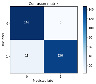
print("Recall rate:",cnf_matrix[1,1]/(cnf_matrix[1,0]+cnf_matrix[1,1]))
class_names = [0,1]
plt.figure()
plot_confusion_matrix(cnf_matrix,
                     classes=class_names,
                     title='Confusion matrix')
plt.show()

Recall rate: 0.9251700680272109

Ir = LogisticRegression(C=best_c,penalty='l2')
Ir.fit(X_train_undersample,y_train_undersample.values.ravel())
y_pred = Ir.predict(X_test.values)

cnf_matrix = confusion_matrix(y_test,y_pred)
np.set_printoptions(precision=2)
print("Recall rate of the model applied to the original data:",cnf_matrix[1,1]/(cnf_matrix[1,0]+cnf_matrix[1,1]))
class_names = [0,1]
plt.figure()
plot_confusion_matrix(cnf_matrix,
                     classes=class_names,
                     title='Confusion matrix')
plt.show()

Recall rate of model applied to original data: 0.9319727891156463

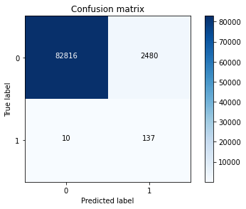
Analysis: the lower left corner indicates that the number of missing classified Neg data is acceptable, while the number in the upper right corner indicates that there are too many wrong classified Neg data, which needs to be corrected!

Correction strategy

1. Model adjustment parameters / optimization algorithm?
   Positive solution: start from the data level, and consider the oversampling scheme that has not been considered before

Effect of classification threshold on results

Ir = LogisticRegression(C=best_c,penalty='l2')
Ir.fit(X_train_undersample,y_train_undersample.values.ravel())
y_pred_undersample_proba = Ir.predict_proba(X_test_undersample.values)
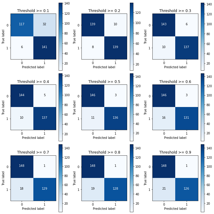
thresholds = [0.1,0.2,0.3,0.4,0.5,0.6,0.7,0.8,0.9]
plt.figure(figsize=(10,10))
j = 1
for i in thresholds:
    y_test_predictions_high_recall = y_pred_undersample_proba[:,1] > i
    plt.subplot(3,3,j)
    j+=1
    cnf_matrix = confusion_matrix(y_test_undersample,y_test_predictions_high_recall)      
    np.set_printoptions(precision=2)
    print("Recall metric in the testing dataset: ", cnf_matrix[1,1]/(cnf_matrix[1,0]+cnf_matrix[1,1]))
    class_names = [0,1]
    plot_confusion_matrix(cnf_matrix,
                         classes=class_names,
                         title="Threshold >= %s"%i)

Recall metric in the testing dataset:  0.9591836734693877
Recall metric in the testing dataset:  0.9455782312925171
Recall metric in the testing dataset:  0.9319727891156463
Recall metric in the testing dataset:  0.9319727891156463
Recall metric in the testing dataset:  0.9251700680272109
Recall metric in the testing dataset:  0.891156462585034
Recall metric in the testing dataset:  0.8775510204081632
Recall metric in the testing dataset:  0.8707482993197279
Recall metric in the testing dataset:  0.8571428571428571

The confusion matrix can be remembered as follows:

Top left: pursue the largest (represents the sample classified as true and correct)

Top right: the sample that pursues the smallest (representing the sample classified as false error) classification error and manslaughter

Bottom right: pursue the largest (represents the correct sample classified as false)

Bottom left: pursue the smallest sample (representing the sample classified as true error) and the sample picked up by classification error

Oversampling strategy

Generate insufficient samples by yourself

SMOTE data generation

Specific process

1. For each sample in the minority, the distance from it to all samples in the minority sample set is calculated by Euclidean distance, and the nearest neighbor samples are sorted
2. Set a sampling ratio N according to the unbalanced proportion of samples. For each small number of samples x, select N samples successively from their nearest neighbors
3. For each selected nearest neighbor sample, a new sample data is constructed with the original sample according to the formula.

• One sentence summary: first find the nearest similar samples, and then take the random number in 0.1 as the proportion on the basis of their distance and add it to the original data points to become a new abnormal sample.

# Oversampling, using smote algorithm to generate samples
# Introducing logistic regression model
# Load data
data = pd.read_csv("creditcard.csv")
 
# The characteristic value of Amount is too large. Normalize it
data['normAmount'] = StandardScaler().fit_transform(data['Amount'].values.reshape(-1, 1))
# Delete the useless Time column and the original Amount column
data = data.drop(['Time', 'Amount'], axis=1)
 
# Get the characteristic column, all rows, and the column name is not a Class column
features = data.loc[:, data.columns != 'Class']
 
# Get the label column, all rows, and the column name is the column of Class
labels = data.loc[:, data.columns == 'Class']
 
# Separate training set and test set
features_train, features_test, labels_train, labels_test = train_test_split(features, labels, test_size=0.2, random_state=0)

from imblearn.over_sampling import SMOTE
oversampler = SMOTE(random_state=0)
os_features,os_labels=oversampler.fit_resample(features_train,labels_train)
os_features = pd.DataFrame(os_features)
os_labels = pd.DataFrame(os_labels)
best_c = printing_Kfold_scores(os_features,os_labels)

==================
Regularization penalty: 0.01
==================

Iteration 1 :recall  =  0.9161290322580645
Iteration 2 :recall  =  0.9144736842105263
Iteration 3 :recall  =  0.9105676662609273
Iteration 4 :recall  =  0.8931754981809389
Iteration 5 :recall  =  0.893626141721898

Average recall rate: 0.905594404526471

==================
Regularization penalty: 0.1
==================

Iteration 1 :recall  =  0.9161290322580645
Iteration 2 :recall  =  0.9144736842105263
Iteration 3 :recall  =  0.9115857032200951
Iteration 4 :recall  =  0.8943295852980293
Iteration 5 :recall  =  0.895120959321177

Average recall rate: 0.9063277928615785

==================
Regularization penalty: 1
==================

Iteration 1 :recall  =  0.9161290322580645
Iteration 2 :recall  =  0.9144736842105263
Iteration 3 :recall  =  0.911807015602523
Iteration 4 :recall  =  0.8945384201096932
Iteration 5 :recall  =  0.8952528549917016

Average recall rate: 0.9064402014345017

==================
Regularization penalty: 10
==================

Iteration 1 :recall  =  0.9161290322580645
Iteration 2 :recall  =  0.9144736842105263
Iteration 3 :recall  =  0.9118734093172512
Iteration 4 :recall  =  0.8945713940273244
Iteration 5 :recall  =  0.8952528549917016

Average recall rate: 0.9064600749609737

==================
Regularization penalty: 100
==================

Iteration 1 :recall  =  0.9161290322580645
Iteration 2 :recall  =  0.9144736842105263
Iteration 3 :recall  =  0.9118734093172512
Iteration 4 :recall  =  0.8945713940273244
Iteration 5 :recall  =  0.8952638462975786

Average recall rate: 0.906462273222149

>>>>>>>>>>>>>>>>>>>>>>>>>>>>>>>
Parameters selected for the best model= 100.0
>>>>>>>>>>>>>>>>>>>>>>>>>>>>>>>

Ir = LogisticRegression(C=best_c,penalty='l2')
Ir.fit(os_features,os_labels.values.ravel())
y_pred = Ir.predict(features_test.values)
cnf_matrix = confusion_matrix(labels_test,y_pred)
np.set_printoptions(precision=2)

print("Confusion matrix:",cnf_matrix[1,1]/(cnf_matrix[1,0]+cnf_matrix[1,1]))

class_names = [0,1]
plt.figure()
plot_confusion_matrix(cnf_matrix,
                     classes=class_names,
                     title="confusion matrix")
plt.show()

Confusion matrix: 0.9405940594059405

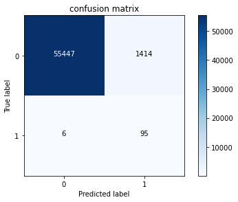
It is found that the proportion of miscarriage of the model results has greatly decreased this time, because more data information can be used, which makes the model more in line with the actual task requirements. For different tasks and data sources, there is no invariable answer, and any results need to be verified.

summary

1. Before starting the task, first check the data and find out what is wrong with the data
2. Put forward a variety of schemes for the problem, and compare these schemes to find the most appropriate scheme to solve the problem
3. Before modeling, the data needs to be processed, such as data standardization, missing value processing, etc
4. First select the evaluation method before modeling, because modeling cannot get the best result at one time. You must try it many times. You need an appropriate evaluation scheme. You can use the general methods: recall rate and accuracy rate, or you can specify the appropriate evaluation criteria according to the actual problems
5. Select the appropriate algorithm
6. For model parameter adjustment, consult the API document before parameter adjustment to know the meaning of each parameter
7. The test results cannot represent the final results. We must apply the established model to the original data.