Pandas Library

Introduction

Numpy performs well in vectorized numerical calculations
But when dealing with more flexible and complex data tasks:
Such as adding labels to data, dealing with missing values, grouping and PivotTables
Numpy seems powerless
The Pandas Library Based on Numpy provides advanced data structure and operation tools that make data analysis faster and simpler

11.1 object creation

11.1.1 Pandas Series object

Series is a one-dimensional array of labeled data

Creation of Series objects

General structure: PD Series(data, index=index, dtype=dtype)
Data: data, which can be a list, dictionary or Numpy array
Index: index, an optional parameter
dtype: data type; optional parameter

1 create with list

• index defaults to integer sequence

import pandas as pd


data = pd.Series([1.5, 3, 4.5, 6])
print(data)

0 1.5
1 3.0
2 4.5
3 6.0
dtype: float64

• Add index

data = pd.Series([1.5, 3, 4.5, 6], index=["a", "b", "c", "d"])
print(data)

a 1.5
b 3.0
c 4.5
d 6.0
dtype: float64

• Add data type
  By default, it is automatically judged from the incoming data

data = pd.Series([1, 2, 3, 4], index=["a", "b", "c", "d"], dtype=float)
print(data)

a 1.0
b 2.0
c 3.0
d 4.0
dtype: float64

Note: data supports multiple data types

data = pd.Series([1, 2, "3", 4], index=["a", "b", "c", "d"])
print(data)

a 1
b 2
c 3
d 4
dtype: object

print(data["a"])
print(data["c"])

1
3

The data type can be forcibly changed

data = pd.Series([1, 2, "3", 4], index=["a", "b", "c", "d"], dtype=float)
print(data)

a 1.0
b 2.0
c 3.0
d 4.0
dtype: float64

print(data["c"])

3.0

If it is not castable, an error will be reported

data = pd.Series([1, 2, "a", 4], index=["a", "b", "c", "d"], dtype=float)
print(data)

2 create with one-dimensional Numpy array

import pandas as pd
import numpy as np

x = np.arange(5)
y = pd.Series(x)
print(y)

0 0
1 1
2 2
3 3
4 4
dtype: int32

3 create with dictionary

• The default key is index and the value is data

population_dict = {"BeiJing": 2154,
                   "ShangHai": 2424,
                   "ShenZhen": 1303,
                   "HangZhou": 981 }
population = pd.Series(population_dict)
print(population)

BeiJing 2154
ShangHai 2424
ShenZhen 1303
HangZhou 981
dtype: int64

• When creating a dictionary, if index is specified, it will be filtered from the keys in the dictionary. If it cannot be found, the value will be set to NaN

population = pd.Series(population_dict, index=["BeiJing", "HangZhou", "c", "d"])
print(population)

BeiJing 2154.0
HangZhou 981.0
c NaN
d NaN
dtype: float64

4. When data is scalar

print(pd.Series(5, index=[100, 200, 300]))

100 5
200 5
300 5
dtype: int64

11.1. 2. Pandas dataframe object

DataFrame is a multidimensional array of labeled data

Creation of DataFrame object

General structure: PD DataFrame(data, index=index, columns=columns)
Data: data, which can be a list, dictionary or Numpy array
Index: index, an optional parameter
columns: column label, optional parameter

1 create through Series objects

population_dict = {"BeiJing": 2154,
                   "ShangHai": 2424,
                   "ShenZhen": 1303,
                   "HangZhou": 981}
population = pd.Series(population_dict)
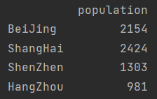
print(pd.DataFrame(population))

print(pd.DataFrame(population, columns=["population"]))

2 create through Series object dictionary

population_dict = {"BeiJing": 2154,
                   "ShangHai": 2424,
                   "ShenZhen": 1303,
                   "HangZhou": 981}
population = pd.Series(population_dict)
GDP_dict = {"BeiJing": 30320,
            "ShangHai": 32680,
            "ShenZhen": 24222,
            "HangZhou": 13468}
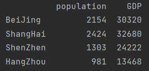
GDP = pd.Series(GDP_dict)
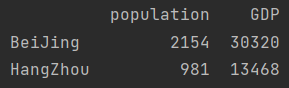
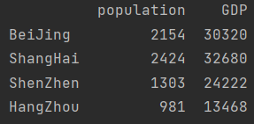
print(pd.DataFrame({"population": population,
                    "GDP": GDP}))

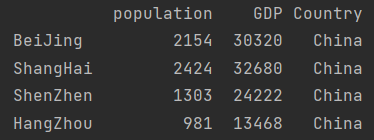
Note: if the quantity is insufficient, it will be supplemented automatically

print(pd.DataFrame({"population": population,
                    "GDP": GDP,
                    "Country": "China"}))

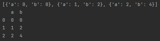
3 create through dictionary list object

• The dictionary index is used as index and the dictionary key is used as columns

data = [{"a": i, "b": 2*i} for i in range(3)]
print(data)
print(pd.DataFrame(data))

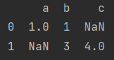
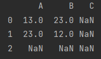
• Keys that do not exist will default to NaN

data = [{"a": 1, "b": 1}, {"b":3, "c": 4}]
print(pd.DataFrame(data))

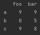
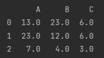
4 created by Numpy two-dimensional array

print(pd.DataFrame(np.random.randint(10, size=(3, 2)), columns=["foo", "bar"], index=["a", "b", "c"]))

11.2 properties of dataframe

11.2. 1 Properties

data = pd.DataFrame({"population":population, "GDP": GDP})
print(data)

1. df.values returns the data represented by the numpy array

print(data.values)

[[ 2154 30320]
[ 2424 32680]
[ 1303 24222]
[ 981 13468]]

2. df.index returns the row index

print(data.index)

Index(['BeiJing', 'ShangHai', 'ShenZhen', 'HangZhou'], dtype='object')

3. df.columns returns the column index

print(data.columns)

Index(['population', 'GDP'], dtype='object')

4. df.shape shape

print(data.shape)

(4, 2)

5. pd.size size

print(data.size)

8

6. pd.dtypes returns the data type of each column

print(data.dtypes)

population int64
GDP int64
dtype: object

11.2. 2 index

1. Get columns

• Dictionary type

print(data["population"])

BeiJing 2154
ShangHai 2424
ShenZhen 1303
HangZhou 981
Name: population, dtype: int64

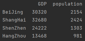
print(data[["GDP", "population"]])  # Multiple columns are obtained in list form

• Object attribute

print(data.GDP)

BeiJing 30320
ShangHai 32680
ShenZhen 24222
HangZhou 13468
Name: GDP, dtype: int64

2. Get row

• Absolute index DF loc

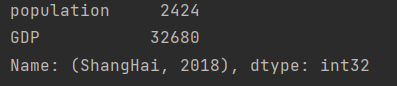
print(data.loc["BeiJing"])

population 2154
GDP 30320
Name: BeiJing, dtype: int64

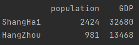
print(data.loc[["BeiJing", "HangZhou"]])

• Relative index

print(data.iloc[0])

population 2154
GDP 30320
Name: BeiJing, dtype: int64

print(data.iloc[[1, 3]])

3. Get scalar

print(data.loc["BeiJing", "GDP"])

30320

print(data.iloc[0, 1])

30320

print(data.values[0][1])

30320

4. Index of series objects

print(type(data.GDP))

<class 'pandas.core.series.Series'>

print(GDP["BeiJing"])

30320

11.2. 3 slice

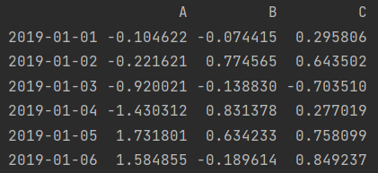
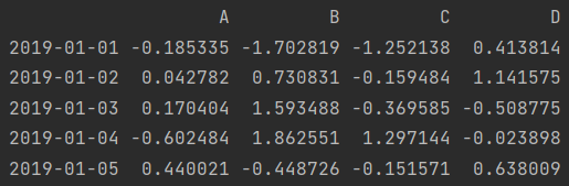
dates = pd.date_range(start='2019-01-01', periods=6)
print(dates)

DatetimeIndex(['2019-01-01', '2019-01-02', '2019-01-03', '2019-01-04',
'2019-01-05', '2019-01-06'],
dtype='datetime64[ns]', freq='D')

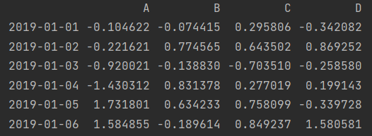
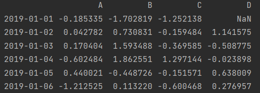
df = pd.DataFrame(np.random.randn(6, 4), index=dates, columns=["A", "B", "C", "D"])
print(df)

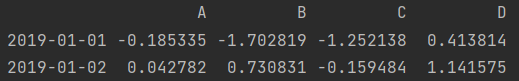
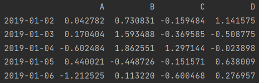
1. Row slicing

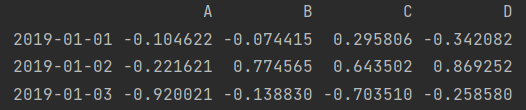
print(df["2019-01-01": "2019-01-03"])
print(df.loc["2019-01-01": "2019-01-03"])
print(df.iloc[0:3])  # End position not included

2. Column slicing

print(df.loc[:, "A": "C"])
print(df.iloc[:, 0: 3])

3. Various values

• Row and column slicing at the same time

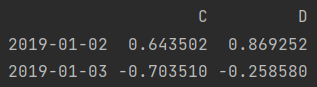
print(df.loc["2019-01-02": "2019-01-03", "C": "D"])  # Row and column simultaneous slicing
print(df.iloc[1: 3, 2:])

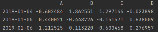
• Row slice, column scatter value

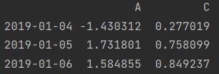
print(df.loc["2019-01-04": "2019-01-06", ["A", "C"]])  # Row slice, column scatter value
print(df.iloc[3:, [0, 2]])

• Row scatter value, column slice

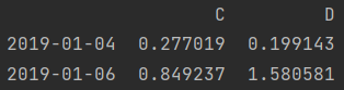
print(df.loc[["2019-01-04", "2019-01-06"], "C": "D"])  # Row scatter value, column slice
print(df.iloc[[3, 5], 2:])

• Row and column values are scattered

print(df.loc[["2019-01-04", "2019-01-06"], ["C", "D"]])  # Row and column values are scattered
print(df.iloc[[3, 5], [2, 3]])

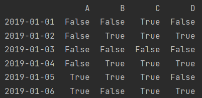
11.2. 4 Boolean index

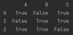
print(df)

print(df > 0)

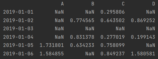
print(df[df > 0])

print(df.A > 0)

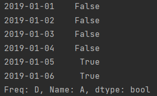
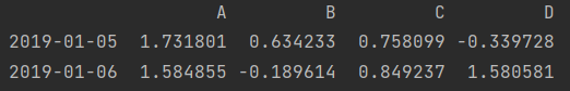
print(df[df.A > 0])

• isin() method

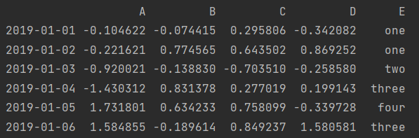
df2 = df.copy()
df2['E'] = ['one', 'one', 'two', 'three', 'four', 'three']
print(df2)

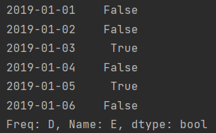
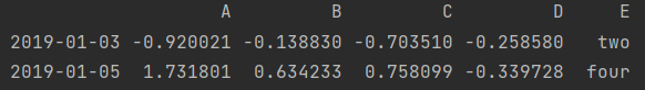
ind = df2['E'].isin(["two", "four"])
print(ind)
print(df2[ind])

11.2. 5 assignment

print(df)

• Add new column to DataFrame

s1 = pd.Series([1, 2, 3, 4, 5, 6], index=pd.date_range('20190101', periods=6))
print(s1)

2019-01-01 1
2019-01-02 2
2019-01-03 3
2019-01-04 4
2019-01-05 5
2019-01-06 6
Freq: D, dtype: int64

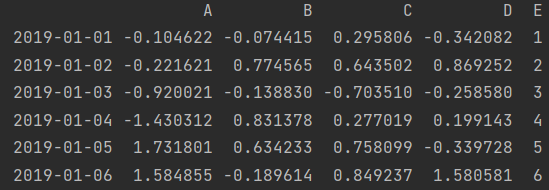
df['E'] = s1
print(df)

• Modify assignment

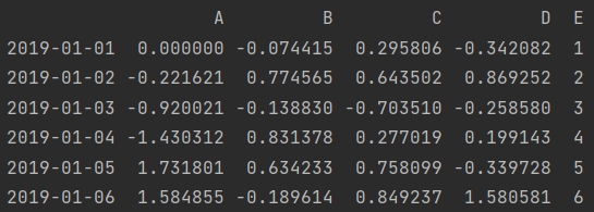
df.loc["2019-01-01", "A"] = 0
print(df)

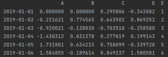
df.iloc[0, 1] = 0
print(df)

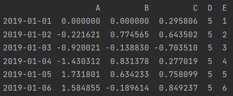
df["D"] = np.array([5]*len(df))  # It can be simplified to df["D"] = 5
print(df)

• Modify index and columns

df.index = [i for i in range(len(df))]
df.columns = [i for i in range(df.shape[1])]
print(df)

11.3 numerical calculation and statistical analysis

11.3. 1. View data

dates = pd.date_range(start='2019-01-01', periods=6)
df = pd.DataFrame(np.random.randn(6, 4), index=dates, columns=["A", "B", "C", "D"])
print(df)

1. View the previous line

print(df.head())  # Default 5 lines

print(df.head(2))

2. View the following lines

print(df.tail())  # Default 5 lines

print(df.tail(3))

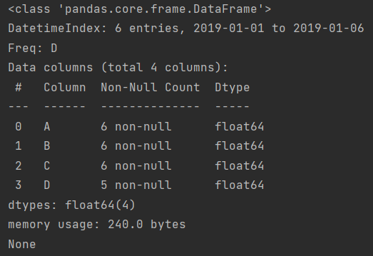
3. View general information
In order to view the overall information, we first change one of the elements to NaN

df.iloc[0, 3] = np.nan
print(df)

print(df.info())

11.3.2 Numpy general function is also applicable to Pandas

1 vectorization operation

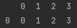
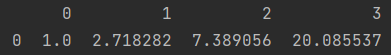
x = pd.DataFrame(np.arange(4).reshape(1, 4))
print(x)

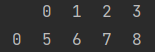
print(x + 5)

print(np.exp(x))

y = pd.DataFrame(np.arange(4, 8).reshape(1, 4))
print(x * y)

2 matrix operation

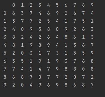
np.random.seed(42)
x = pd.DataFrame(np.random.randint(10, size=(10, 10)))
print(x)

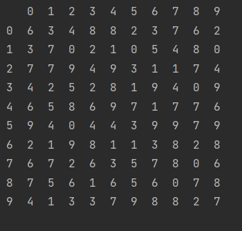
• Transpose

z = x.T
print(z)

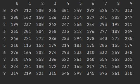
• Matrix multiplication

np.random.seed(1)
y = pd.DataFrame(np.random.randint(10, size=(10, 10)))
print(x.dot(y))

We can use the% timeit method to compare the time required for the next two kinds of multiplication

%timeit x.dot(y)
%timeit np.dot(x, y)

NP can be found Dot (x, y) takes less time

• Perform the same operation, comparison between Numpy and Pandas

In general, pure computing is faster in Numpy
Numpy focuses more on calculation and Pandas focuses more on data analysis

3 broadcast operation

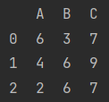
np.random.seed(42)
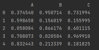
x = pd.DataFrame(np.random.randint(10, size=(3, 3)), columns=list("ABC"))
print(x)

• Spread by line

print(x.iloc[0])

A 6
B 3
C 7
Name: 0, dtype: int32

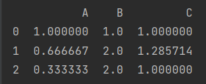
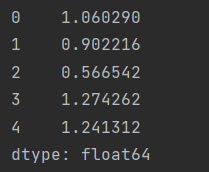
print(x/x.iloc[0])

• Column propagation

print(x.div(x.A, axis=0))  # add sub div mul

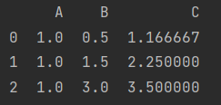
Here, if axis is set to 1, it means propagation by column. You can also explicitly write out that axis=0 means propagation by row.

11.3. 3 new usage

1 Index alignment

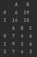
np.random.seed(42)
A = pd.DataFrame(np.random.randint(0, 20, size=(2, 2)), columns=list("AB"))
B = pd.DataFrame(np.random.randint(0, 10, size=(3, 3)), columns=list("ABC"))
print(A)
print(B)

• Pandas will automatically align the indexes of the two objects, and NP. Is used for values without Nan representation

print(A+B)

• The default value can be filled with fill value

print(A.add(B, fill_value=0))

2 statistical correlation

• Data type statistics

y = np.random.randint(3, size=20)
print(y)

[2 0 2 2 0 0 2 1 2 2 2 2 0 2 1 0 1 1 1 1]

print(np.unique(y))

[0 1 2]

from collections import Counter
print(Counter(y))

Counter({2: 9, 1: 6, 0: 5})

y1 = pd.DataFrame(y, columns=["A"])
print(y1)

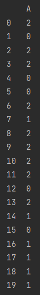
print(np.unique(y1))

[0 1 2]

print(y1["A"].value_counts())

2 9
1 6
0 5
Name: A, dtype: int64

• Generate new results and sort them

population_dict = {"BeiJing": 2154,
                   "ShangHai": 2424,
                   "ShenZhen": 1303,
                   "HangZhou": 981}
population = pd.Series(population_dict)
GDP_dict = {"BeiJing": 30320,
            "ShangHai": 32680,
            "ShenZhen": 24222,
            "HangZhou": 13468}
GDP = pd.Series(GDP_dict)
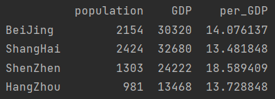
city_info = pd.DataFrame({"population": population, "GDP": GDP})
print(city_info)

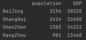
city_info["per_GDP"] = city_info["GDP"]/city_info["population"]
print(city_info)

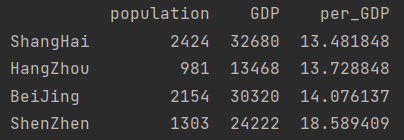
sort ascending

print(city_info.sort_values(by="per_GDP"))

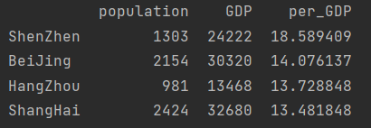
sort descending

print(city_info.sort_values(by="per_GDP", ascending=False))

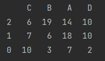
Sort by axis

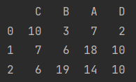
data = pd.DataFrame(np.random.randint(20, size=(3, 4)), index=[2, 1, 0], columns=list("CBAD"))
print(data)

Row sorting

print(data.sort_index())

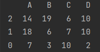
Column sorting

print(data.sort_index(axis=1))

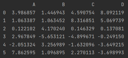
• statistical method

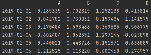
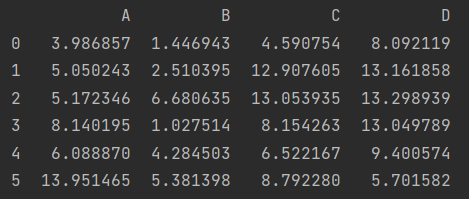
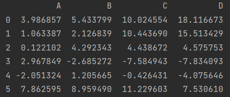
df = pd.DataFrame(np.random.normal(2, 4, size=(6, 4)), columns=list("ABCD"))
print(df)

Non empty number

df.count()

A 6
B 6
C 6
D 6
dtype: int64

Summation (default summation of columns)

df.sum()

A 13.951465
B 5.381398
C 8.792280
D 5.701582
dtype: float64

df.sum(axis=1)  # Sum of rows

0 18.116673
1 15.513429
2 4.575753
3 -7.834093
4 -4.075646
5 7.530610
dtype: float64

Max min

df.min()  # Default minimum value of each column

A -2.051324
B -5.653121
C -4.899671
D -3.698993
dtype: float64

df.max(axis=1)  # Maximum value of each row after shaft replacement 

0 8.092119
1 8.316851
2 4.170240
3 2.967849
4 3.256989
5 7.862595
dtype: float64

print(df.idxmax())  # Maximum coordinates

A 5
B 2
C 1
D 0
dtype: int64

mean value

df.mean()

A 2.325244
B 0.896900
C 1.465380
D 0.950264
dtype: float64

variance

df.var()

A 11.887325
B 11.911567
C 21.841270
D 22.569365
dtype: float64

standard deviation

df.std()

A 3.447800
B 3.451314
C 4.673464
D 4.750723
dtype: float64

median

df.median()

A 2.015618
B 1.271919
C 1.208221
D -0.056035
dtype: float64

Mode

data = pd.DataFrame(np.random.randint(5, size=(10, 2)), columns=list("AB"))
print(data)

data.mode()

75% quantile

df.quantile(0.75)

A 3.732105
B 2.804478
C 4.010594
D 3.836574
Name: 0.75, dtype: float64

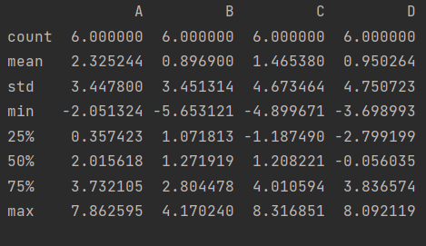
catch all in one draft

df.describe()

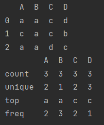
The character type also has a describe

data_2 = pd.DataFrame([["a", "a", "c", "d"],
                       ["c", "a", "c", "b"],
                       ["a", "a", "d", "c"]], columns=list("ABCD"))
print(data_2)
print(data_2.describe())

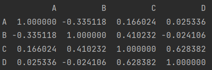
Correlation coefficient and covariance

print(df.corr())

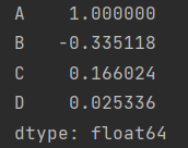
print(df.corrwith(df["A"]))

Custom output
Usage of apply(method): use the method to perform corresponding operations on each column by default

df.apply(np.cumsum)

print(df.apply(np.cumsum, axis=1))

df.apply(sum)

A 13.951465
B 5.381398
C 8.792280
D 5.701582
dtype: float64

df.apply(lambda x: x.max()-x.min())

A 9.913920
B 9.823361
C 13.216523
D 11.791112
dtype: float64

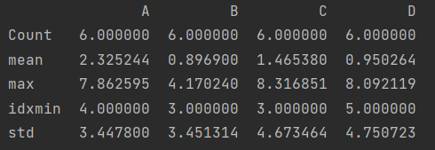
def my_describe(x):
    return pd.Series([x.count(), x.mean(), x.max(), x.idxmin(), x.std()], \
                     index=["Count", "mean", "max", "idxmin", "std"])


print(df.apply(my_describe))

11.4 missing value handling

11.4. 1 missing value found

import pandas as pd
import numpy as np

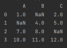
data = pd.DataFrame(np.array([[1, np.nan, 2],
                              [np.nan, 3, 4],
                              [5, 6, None]]), columns=["A", "B", "C"])
print(data)

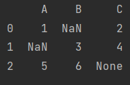
Note: there are None, string, etc. the data type is changed to object, which consumes more resources than int and float

data.dtypes

A object
B object
C object
dtype: object

data.isnull()

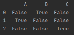
data.notnull()

11.4. 2 delete missing values

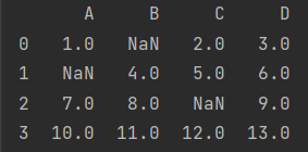
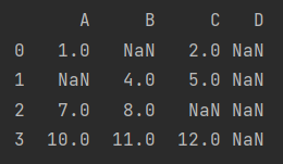
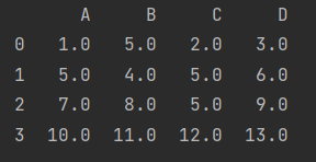
data = pd.DataFrame(np.array([[1, np.nan, 2, 3],
                              [np.nan, 4, 5, 6],
                              [7, 8, np.nan, 9],
                              [10, 11, 12, 13]]), columns=["A", "B", "C", "D"])
print(data)

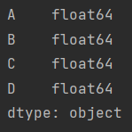
Note: NP Nan is a special floating point number

data.dtypes

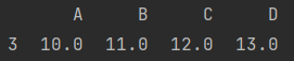
1. Delete the whole line

data.dropna()

2. Delete the whole column

data.dropna(axis="columns")

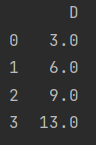
data["D"] = np.nan
print(data)

data.dropna(axis="columns", how="all")  # Delete when all elements are missing. any means delete when there is a missing element

11.4. 3 fill in missing values

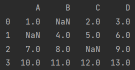
data.fillna(value=5)

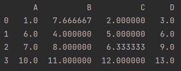
• Replace with mean

fill = data.mean()
print(data.fillna(value=fill))

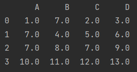
If all average values are used instead, the average value can be taken after stack leveling

fill = data.stack().mean()
print(data.fillna(value=fill))

11.5 consolidated data

• Construct a function to produce DataFrame

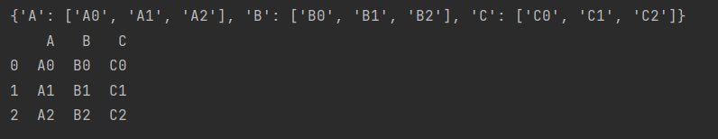
def make_df(cols, ind):
    """A simple DataFrame"""
    data = {c: [str(c)+str(i) for i in ind] for c in cols}
    print(data)
    return pd.DataFrame(data, ind)


make_df("ABC", range(3))

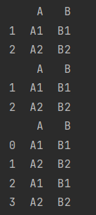
• Vertical merge
  If the row labels overlap, the overlapping row labels are retained

df_1 = make_df("AB", [1, 2])
df_2 = make_df("AB", [3, 4])
print(df_1)
print(df_2)

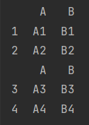
print(pd.concat([df_1, df_2]))

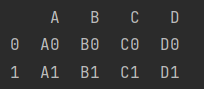
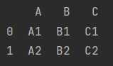
• Horizontal merge
  If the column labels overlap, the overlapping column labels are retained

df_3 = make_df("AB", [0, 1])
df_4 = make_df("CD", [0, 1])
print(df_3)
print(df_4)

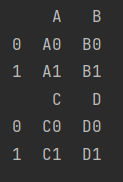
print(pd.concat([df_3, df_4], axis=1))

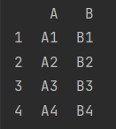
• Index overlap
  When labels overlap, we sometimes want labels to be rearranged, so we need to add the parameter ignore_index=True

df_5 = make_df("AB", [1, 2])
df_6 = make_df("AB", [1, 2])
print(df_5)
print(df_6)
print(pd.concat([df_5, df_6], ignore_index=True))

The same is true for column overlap. Add the parameter axis=1

• Align merge()
  merge() can be used to merge when there are corresponding same values (common columns)

df_9 = make_df("AB", [1, 2])
df_10 = make_df("BC", [1, 2])
print(df_9)
print(df_10)

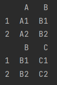
We can see column B in df_9 and DF_ The correspondence in 10 is equal. We want column B to remain unchanged when merging

print(pd.merge(df_9, df_10))

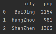
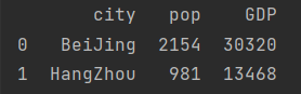
[example] merge city information

population_dict = {"city": ("BeiJing", "HangZhou", "ShenZhen"),
                   "pop": (2154, 981, 1303)}
population = pd.DataFrame(population_dict)
print(population)

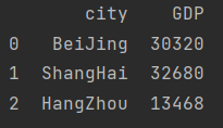
GDP_dict = {"city": ("BeiJing", "ShangHai", "HangZhou"),
            "GDP": (30320, 32680, 13468)}
GDP = pd.DataFrame(GDP_dict)
print(GDP)

city_info = pd.merge(population, GDP)
print(city_info)

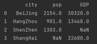
If you don't want to abandon Shanghai and Shenzhen, you need to add parameters

city_info = pd.merge(population, GDP, how="outer")
print(city_info)

11.6 grouping and PivotTables

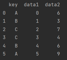
df = pd.DataFrame({"key": ["A", "B", "C", "C", "B", "A"],
                   "data1": range(6),
                   "data2": np.random.randint(0, 10, size=6)})
print(df)

11.6. 1 grouping

• Delay calculation (save first and wait for processing)

df.groupby("key")

<pandas.core.groupby.generic.DataFrameGroupBy object at 0x000001EDFF4444C0>

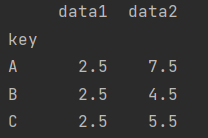
df.groupby("key").sum()

df.groupby("key").mean()

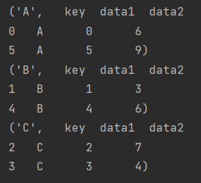
So what exactly is groupby?

for i in df.groupby("key"):
    print(str(i))

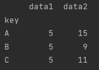
• Value by column

df.groupby("key")["data2"].sum()

key
A 15
B 9
C 11
Name: data2, dtype: int32

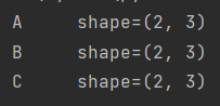
• Iterate by group

for data, group in df.groupby("key"):
    print("{0:5} shape={1}".format(data, group.shape))

• Call method

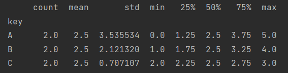
df.groupby("key")["data1"].describe()

• Support for more complex operations

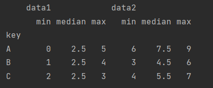
df.groupby("key").aggregate(["min", "median", "max"])

• filter

np.random.seed(1)
df = pd.DataFrame({"key": ["A", "B", "C", "C", "B", "A"],
                   "data1": range(6),
                   "data2": np.random.randint(0, 10, size=6)})
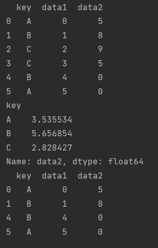
print(df)


def filter_func(x):
    return x["data2"].std() > 3


print(df.groupby("key")["data2"].std())
print(df.groupby("key").filter(filter_func))

• transformation

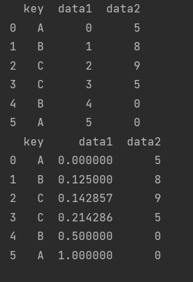
df = pd.DataFrame({"key": ["A", "B", "C", "C", "B", "A"],
                   "data1": range(6),
                   "data2": np.random.randint(0, 10, size=6)})
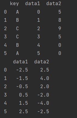
print(df)
print(df.groupby("key").transform(lambda x: x - x.mean()))

• apply method

def norm_by_data2(x):
    x["data1"] /= x["data2"].sum()
    return x

print(df.groupby("key").apply(norm_by_data2))

• Set list and array as grouping key

print(df)
L = [0, 1, 0, 1, 2, 0]
print(df.groupby(L).sum())

• Mapping indexes to groups with dictionaries

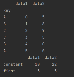
df2 = df.set_index("key")
print(df2)
mapping = {"A": "first", "B": "constant", "C": "constant"}
print(df2.groupby(mapping).sum())

• Any Python function

print(df2.groupby(str.lower).mean())

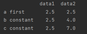
• A list of valid values

print(df2.groupby([str.lower, mapping]).mean())

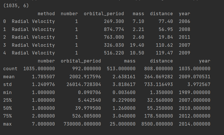
[example 1] planetary observation data processing

import seaborn as sns


planets = sns.load_dataset('planets')
print(planets.shape)  # Get shape
print(planets.head())  # View the first five lines
print(planets.describe())  # statistical information 

Now we hope to realize the observation quantity in different times (decade, unit) under different observation methods by grouping.
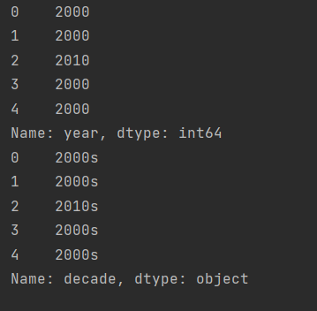
First, we should define the era.

decade = 10 * (planets["year"]//10)
print(decade.head())
decade = decade.astype(str) + "s"
decade.name = "decade"
print(decade.head())

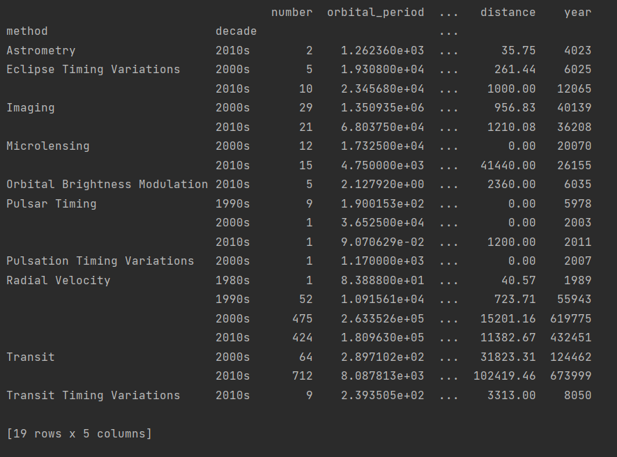
After definition, we group the method and decade.

print(planets.groupby(["method", decade]).sum())

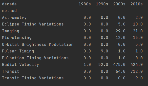
In fact, we only need the data in the column number, so we can propose number separately, expand it with unstack to make it more beautiful, and finally fill the missing value with 0 with fillna.

print(planets.groupby(["method", decade])["number"].sum().unstack().fillna(0))

11.6. 2 PivotTable report

[example 2] analysis of Titanic passenger data

import seaborn as sns


titanic = sns.load_dataset("titanic")
print(titanic.head())
print(titanic.describe())

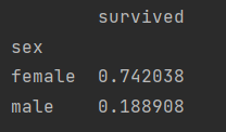
Now we want to get the survival rate of different genders.

print(titanic.groupby("sex")["survived"].mean())

sex
female 0.742038
male 0.188908
Name: survived, dtype: float64

The index "served" is expressed as Series in one bracket and DataFrame in two brackets

print(titanic.groupby("sex")[["survived"]].mean())

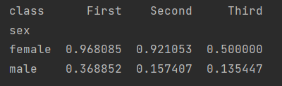
More specifically, we want to see the survival of different cabins under different genders.

print(titanic.groupby(["sex", "class"])["survived"].aggregate("mean").unstack())

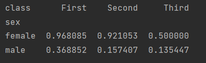
We found that writing by groupby alone is complex and unreadable, but Pandas provides a PivotTable method. Let's take a look at how to use PivotTable to achieve the same function.

print(titanic.pivot_table("survived", index="sex", columns="class"))

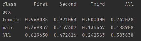
We can find that we can use pivot directly_ The table method returns the average value of data by default.
We can also add other parameters to get different results.
aggfunc to change the method and margins to set the overview.

print(titanic.pivot_table("survived", index="sex", columns="class", aggfunc="mean", margins=True))

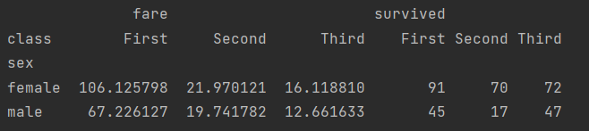
When we use pivot_ If you want to process multiple types of data, you can select the corresponding methods in aggfuc. For example, in this example, we not only want to get the number of survival, but also need the average ticket price.

print(titanic.pivot_table(index="sex", columns="class", aggfunc={"survived": "sum", "fare": "mean"}))

11.7 others

1. Vectorization string operation
2. Processing time series
3. Multilevel index: used for multidimensional arrays

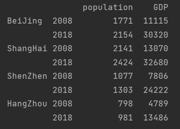
base_data = np.array([[1771, 11115],
                      [2154, 30320],
                      [2141, 13070],
                      [2424, 32680],
                      [1077, 7806],
                      [1303, 24222],
                      [798, 4789],
                      [981, 13486]])
data = pd.DataFrame(base_data, index=[
    ["BeiJing", "BeiJing", "ShangHai", "ShangHai", "ShenZhen", "ShenZhen", "HangZhou", "HangZhou"],
    [2008, 2018] * 4], columns=["population", "GDP"])
print(data)

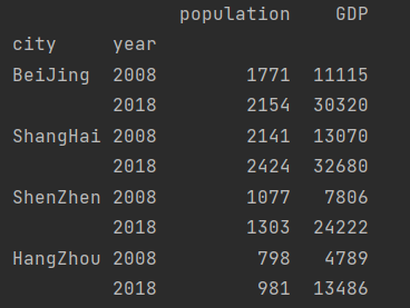
Modify row index name

data.index.names = ["city", "year"]
print(data)

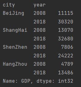
Value of column data

print(data["GDP"])

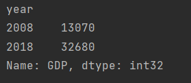
Take GDP of a city

print(data.loc["ShangHai", "GDP"])

Take the situation of a city in a year

print(data.loc["ShangHai", 2018])

1. High performance Pandas: eval()

df1, df2, df3, df4 = (pd.DataFrame(np.random.random((10000,100))) for i in range(4))
%timeit (df1+df2)/(df3+df4)

17.6 ms ± 120 µs per loop (mean ± std. dev. of 7 runs, 100 loops each)

• The memory allocation of the intermediate process of compound algebraic calculation is reduced, and the running speed is improved

%timeit pd.eval("(df1+df2)/(df3+df4)")

10.5 ms ± 153 µs per loop (mean ± std. dev. of 7 runs, 100 loops each)

It can be compared that the operation result is the same

np.allclose((df1+df2)/(df3+df4), pd.eval("(df1+df2)/(df3+df4)"))

True

• Implement inter column operation

df = pd.DataFrame(np.random.random((1000, 3)), columns=list("ABC"))
df.head()

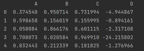
df["D"] = pd.eval("(df.A+df.B)/(df.C-1)")
df.head()

• Use local variables

column_mean = df.mean(axis=1)
res = df.eval("A+@column_mean")
res.head()

1. High performance Pandas: query()

df.head()

%timeit df[(df.A < 0.5) & (df.B > 0.5)]

1.11 ms ± 9.38 µs per loop (mean ± std. dev. of 7 runs, 1000 loops each)

%timeit df.query("(A < 0.5)&(B > 0.5)")

2.55 ms ± 199 µs per loop (mean ± std. dev. of 7 runs, 100 loops each)

Instead, the time becomes longer. The reason is that the amount of data is too small, resulting in the high time cost of calling the method itself

1. Use timing of eval() and query()
   When the array is small, the normal method is faster
   Therefore, when the amount of data is large, eval and query are called to improve the running speed

df.values.nbytes

32000

df1.values.nbytes

8000000

The above is the in-depth exploration in section 11. Pandas is an advanced tool that focuses more on data analysis.
The next section takes a closer look at the Matplotlib library.