In the previous article, the blogger introduced a model reflecting the relationship between two variables, namely, one variable linear regression model. If there are several variables, then we need to use multiple linear regression model.
First, import related modules and datasets:

from sklearn import model_selection
import pandas as pd
import numpy as np
import statsmodels.api as sm

data=pd.read_excel(r'/Users/fangluping/Desktop/Influencing factors of housing sales/Wangchao Mansion.xlsx',
                   usecols=['House type configuration','Predicted building area','Total price','Unit price of construction surface'],skipfooter=1)
data.head()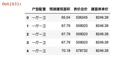

    #Split data set into training set and test set
train, test = model_selection.train_test_split(data, test_size = 0.2, random_state=1234)

#Modeling based on train data set
model=sm.formula.ols('Total price~Predicted building area+Unit price of construction surface+C(House type configuration)',data=data).fit()
print('The partial regression coefficients of the model are as follows:',model.params)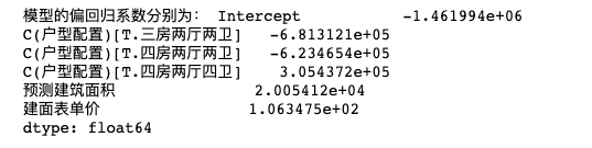

Compare the predicted value with the actual value:

#Delete the sales status variable in the test data set and forecast with the remaining independent variables
test_X = test.drop(labels = 'Total price', axis = 1)
pred = model.predict(exog = test_X)

pd.DataFrame({'Forecast':pred,'Actual':test.Total price})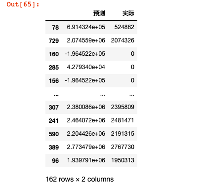

Because the "house type configuration" variable is discrete, python model will automatically convert it into several dummy variables. Then these new dummy variables have a high correlation, that is, when a house type is one hall and one bathroom, it cannot be three rooms, two halls and two bathrooms, so the model will automatically remove one of the variables, such as one hall and one bathroom.
If we don't want the model to be automatically eliminated, can we manually eliminate it ourselves?
The answer, of course, is yes:

# Generate dummy variable derived from house type configuration variable
dummies = pd.get_dummies(data.House type configuration)
# Merge dummy variables horizontally with the original dataset
data_New = pd.concat([data,dummies], axis = 1)
# Delete the house type configuration variable and the variable of three rooms, two halls and two bathrooms (because the house type configuration variable has been decomposed into dummy variable, the variable of three rooms, two halls and two bathrooms needs to be used as reference group)
data_New.drop(labels = ['House type configuration','Three rooms, two halls and two bathrooms'], axis = 1)
# Split data set
train, test = model_selection.train_test_split(data_New, test_size = 0.2, random_state=1234)
# modeling
model2 = sm.formula.ols('Total price~Predicted building area+Unit price of construction surface+One hall and one bathroom+Four rooms, two halls and four bathrooms+Four rooms, two halls and two bathrooms', data = train).fit()
print('The partial regression coefficients of the model are as follows:\n', model2.params)

The coefficients generated this time are as follows: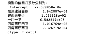

In addition, python can generate the correlation coefficient between variables with one key:

data.drop('House type configuration',axis=1).corrwith(data['Total price'])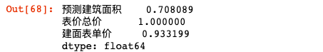

data.drop('House type configuration',axis=1).corr()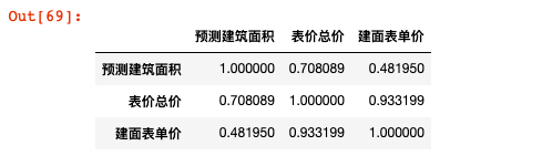

After the model is built, let's check the accuracy of the model. We use F test to test the model and t test to test the parameters

#F-test of the model
import numpy as np

#Calculating the mean value of dependent variables in modeling data
ybar=train.Total price.mean()

#Number of statistical variables and number of observations
p=model2.df_model
n=train.shape[0]

#Calculate the sum of squares of regression dispersion
RSS=np.sum((model2.fittedvalues-ybar)**2)

#Sum of squares of calculation errors
ESS=np.sum(model2.resid**2)

#Calculate the value of F statistic
F=(RSS/p)/(ESS/(n-p-1))

print('F Value of statistic:',F)
#Comparison results
from scipy.stats import f

#Calculating the theoretical value of F distribution
F_Theory=f.ppf(q=0.95,dfn=p,dfd=n-p-1)
print('F The theoretical value of the distribution is:',F_Theory)

There is a big difference between the two F values, indicating that the coefficients of each variable are not all equal to 0, that is, this model can be used.
Another line of code verifies the following parameters:

#t test
model2.summary()

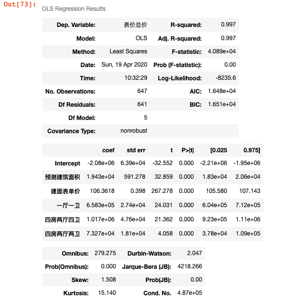
We see that the value of p is 0.000, that is, it is less than 0.005, indicating that the total price of the house is related to each variable here.