This paper introduces the data mining of shared single vehicle in detail, including data analysis and model development. It consists of the following steps:

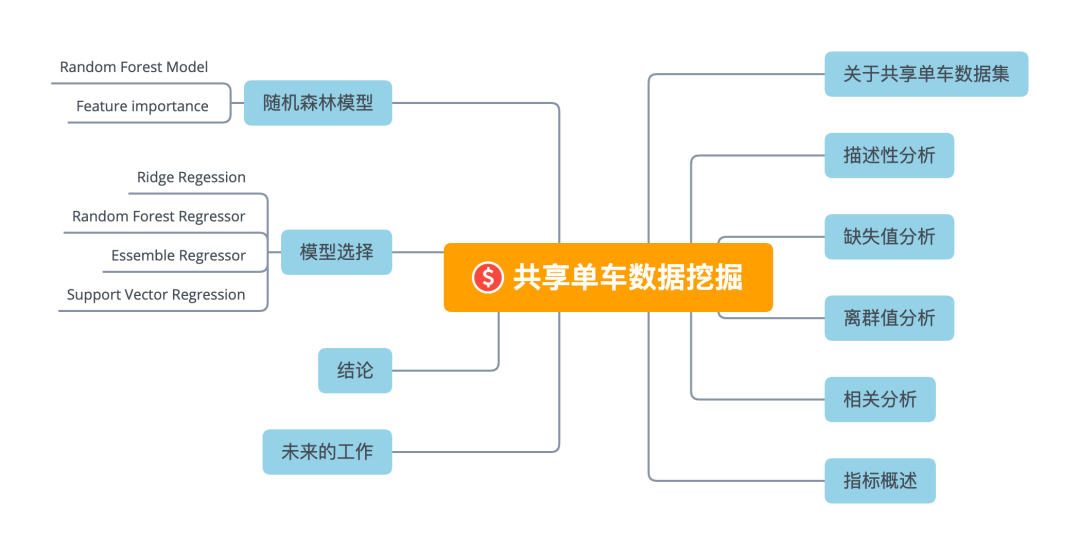
Shared vehicle data mining

Data set introduction

About sharing data sets

Bicycle sharing system is a new generation of traditional bicycle rental. The whole process from registered member, rental to return is automated. Through these systems, users can easily rent bicycles from one specific location and return them at another location. At present, there are more than 500 bike sharing projects around the world, which are composed of more than 500000 bicycles. Today, because of their important role in transportation, environment and health issues, people have great interest in these systems.

In addition to the interesting applications of bicycle sharing systems in the real world, many researchers are interested in the data generated by these systems. Unlike other transportation services (such as buses or subways), the duration, departure time and arrival location of shared bicycles are clearly recorded in the system. This function turns the bicycle sharing system into a virtual sensor network, which can be used to sense the mobility in the city. Therefore, by monitoring these data, it is expected that most important events in the city can be detected.

Today we use these data sets to mine the effective information contained in them. Next, from exploring data attributes, cleaning data, to model development, learn together and make common progress.

Note that this data set is a foreign shared single vehicle data set, not a domestic shared single vehicle data set. But it does not affect our learning of data mining related knowledge and technology.

Attribute information

Both hour.csv and day.csv have the following fields, but there is no hr field in day.csv

• instant: record index
• dteday: Date
• Season: season (1: spring, 2: summer, 3: autumn, 4: winter)
• yr: year (0:2011, 1:2012)
• mnth: month (1 to 12)
• hr: hours (0 to 23)
• Holiday: is it a holiday
• weekday: what day of the week
• workingday: working day. If the day is neither weekend nor holiday, it is 1; otherwise, it is 0.
• weathersit:
  • 1: Sunny, cloudy, partly cloudy, cloudless
  • 2: Mist + cloudy, mist + broken cloud, mist + a small amount of cloud, mist
  • 3: Light snow, light rain + thunderstorm + scattered clouds, light rain + scattered clouds
  • 4: Heavy rain + ice sheet + thunderstorm + fog, snow + fog
• temp: standardized temperature data, in degrees Celsius. These values are obtained by (t-t_min)/(t_max-t_min, t_min=-8, t_max=+39 (only in the hourly range)
• atemp: normal somatosensory temperature in degrees Celsius. These values are obtained by (t-t_min)/(t_max-t_min), t_min=-16, t_max=+50 (only in the hourly range)
• hum: normalized humidity. These values are divided into 100 (maximum)
• windspeed: normalized wind speed data. These values are divided into 67 (maximum)
• casual: number of logged off users
• Registered: number of registered users
• cnt: total number of bicycles rented, including cancelled and registered bicycles

preparation in advance

Import module

import seaborn as sns
import matplotlib.pyplot as plt
from prettytable import PrettyTable
import numpy as np  
import pandas as pd  
from sklearn.model_selection import RandomizedSearchCV
from sklearn.metrics import mean_squared_error, mean_absolute_error, mean_squared_log_error
from sklearn.linear_model import Lasso, ElasticNet, Ridge, SGDRegressor
from sklearn.svm import SVR, NuSVR
from sklearn.ensemble import BaggingRegressor, RandomForestRegressor
from sklearn.neighbors import KNeighborsClassifier
from sklearn.cluster import KMeans
from sklearn.ensemble import RandomForestClassifier
from sklearn.ensemble import GradientBoostingClassifier
from sklearn.linear_model import LinearRegression
import random
%matplotlib inline

random.seed(100)

Define data acquisition function

class Dataloader():
    '''
    Bicycle shared dataset data loader.
    '''
    def __init__(self, csv_path):
        ''' 
        Initialize the bicycle shared dataset data loader.
        param:  csv_path {str} 
        -- Bicycle shared dataset CSV The path to the file.
        '''
        self.csv_path = csv_path
        self.data = pd.read_csv(self.csv_path)
        # Shuffle
        self.data.sample(frac=1.0, replace=True, random_state=1)

    def getHeader(self):
        ''' 
        Get shared bike CSV The column name of the file.
        return:  [list of str]
        --CSV Column name of the file
        '''
        return list(self.data.columns.values)
        
    def getData(self):
        '''   
        Partition training, verification and test sets
        return: pandas DataFrames
        -- Different data sets after division pandas DataFrames
        '''
        # The data were divided into training, verification and test sets in the ratio of 60:20:20
      
        split_train = int(60 / 100 * len(self.data)) 
        split_val = int(80 / 100 * len(self.data)) 
        train = self.data[: split_train]
        val = self.data[split_train: split_val]
        test = self.data[split_val: ]
        return train, val,  test
        
    def getFullData(self):
        ''' 
        In a DataFrames Get all data from.
        return:  pandas DataFrames
        -- Complete shared dataset data
        '''
        return self.data

Descriptive analysis

Partition training, verification and test data sets

dataloader = Dataloader('../data/bike/hour.csv')
train, val, test = dataloader.getData()
fullData = dataloader.getFullData()

category_features = ['season', 'holiday', 'mnth', 'hr',   
                     'weekday', 'workingday', 'weathersit']
number_features = ['temp', 'atemp', 'hum', 'windspeed']

features= category_features + number_features
target = ['cnt']

features

['season',
 'holiday',
 'mnth',
 'hr',
 'weekday',
 'workingday',
 'weathersit',
 'temp',
 'atemp',
 'hum',
 'windspeed']

Get column name of DataFrame:

print(list(fullData.columns))

['instant', 'dteday', 'season', 'yr', 'mnth',
'hr', 'holiday', 'weekday', 'workingday', 
'weathersit', 'temp', 'atemp', 'hum', 
'windspeed', 'casual', 'registered', 'cnt']

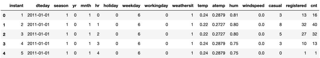
Print the first five examples of the dataset to explore the data:

fullData.head(5)

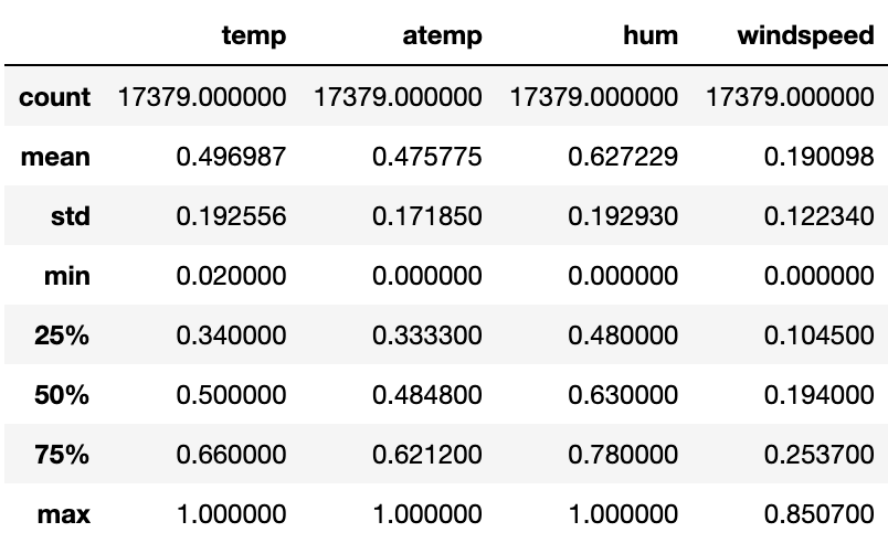
Get data statistics for each column:

fullData[number_features].describe()

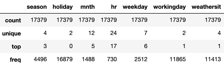
for col in category_features: 
    fullData[col] = fullData[col].astype('category')
fullData[category_features].describe()

Missing value analysis

See previous articles for missing value analysis: Missing value processing, can you really handle it?

Check NULL value in data:

print(fullData.isnull().any())

instant       False
dteday        False
season        False
yr            False
mnth          False
hr            False
holiday       False
weekday       False
workingday    False
weathersit    False
temp          False
atemp         False
hum           False
windspeed     False
casual        False
registered    False
cnt           False
dtype: bool

Outlier analysis

Box diagram

sns.set(font_scale=1.0)
fig, axes = plt.subplots(nrows=3,ncols=2)
fig.set_size_inches(15, 15)
sns.boxplot(data=train,y="cnt",orient="v",ax=axes[0][0])
sns.boxplot(data=train,y="cnt",x="mnth",orient="v",ax=axes[0][1])
sns.boxplot(data=train,y="cnt",x="weathersit",orient="v",ax=axes[1][0])
sns.boxplot(data=train,y="cnt",x="workingday",orient="v",ax=axes[1][1])
sns.boxplot(data=train,y="cnt",x="hr",orient="v",ax=axes[2][0])
sns.boxplot(data=train,y="cnt",x="temp",orient="v",ax=axes[2][1])

axes[0][0].set(ylabel='Count',title="Box Plot On Count")
axes[0][1].set(xlabel='Month', ylabel='Count',title="Box Plot On Count Across Months")
axes[1][0].set(xlabel='Weather Situation', ylabel='Count',title="Box Plot On Count Across Weather Situations")
axes[1][1].set(xlabel='Working Day', ylabel='Count',title="Box Plot On Count Across Working Day")
axes[2][0].set(xlabel='Hour Of The Day', ylabel='Count',title="Box Plot On Count Across Hour Of The Day")
axes[2][1].set(xlabel='Temperature', ylabel='Count',title="Box Plot On Count Across Temperature")

for tick in axes[2][1].get_xticklabels(): 
    tick.set_rotation(90)

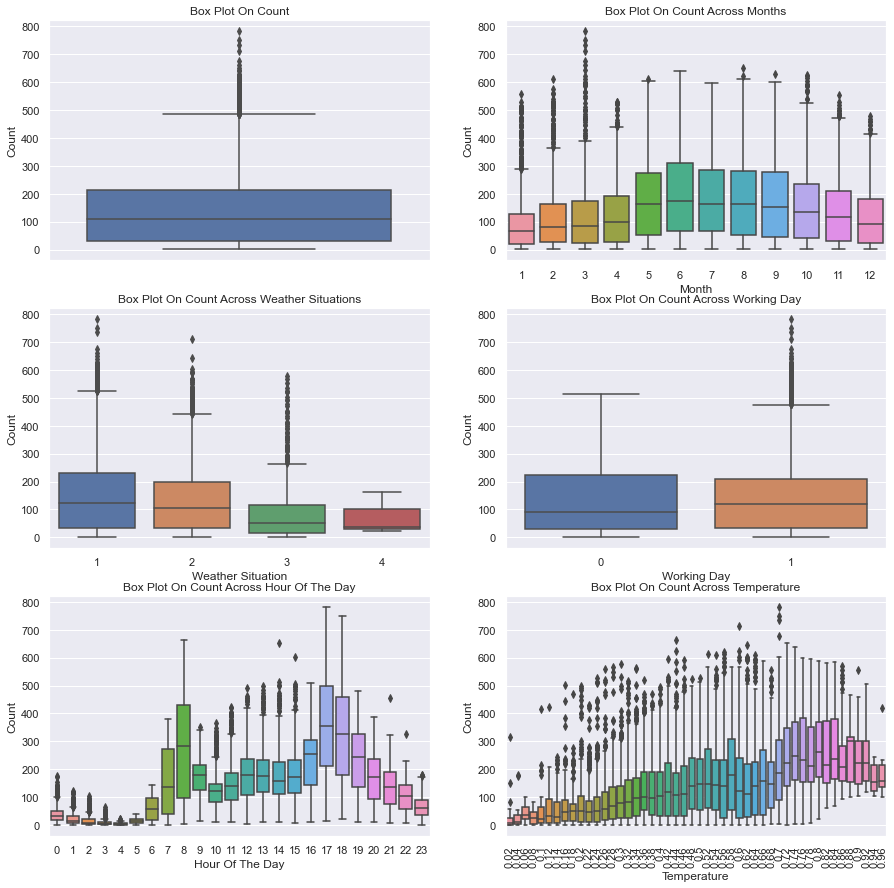
Analysis: the box chart of weekdays and holidays shows that more bicycles are rented on normal weekdays than on weekends or holidays. The box chart per hour shows that the maximum is at 8 a.m. and 5 p.m., indicating that most users of bicycle rental services use bicycles to go to work or school. Another important factor seems to be temperature: higher temperature leads to an increase in the number of bicycles rented The lower temperature not only reduces the average lease quantity, but also shows more outliers in the data.

Remove outliers from data

sns.distplot(train[target[-1]]);

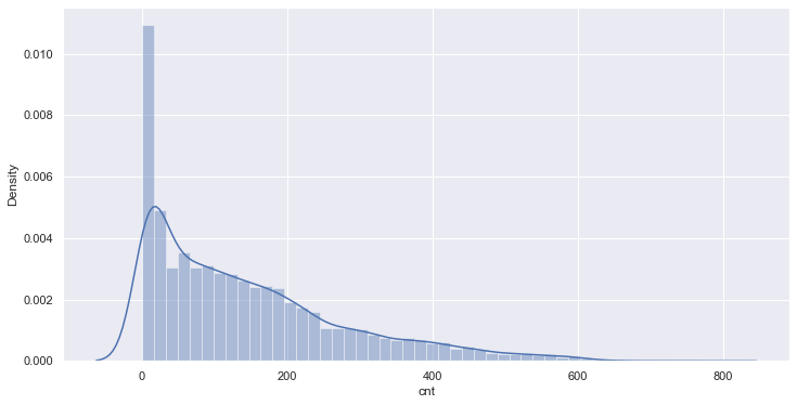
The distribution map of the count value shows that the count value does not conform to the normal distribution. We will use the median and interquartile interval (IQR) to identify and remove abnormal values in the data. (another method is to convert the target value to the normal distribution and use the mean and standard deviation.)

print("Samples in the train set with outliers: {}".format(len(train)))
q1 = train.cnt.quantile(0.25)
q3 = train.cnt.quantile(0.75)
iqr = q3 - q1
lower_bound = q1 -(1.5 * iqr) 
upper_bound = q3 +(1.5 * iqr) 
train_preprocessed = train.loc[(train.cnt >= lower_bound) & (train.cnt <= upper_bound)]
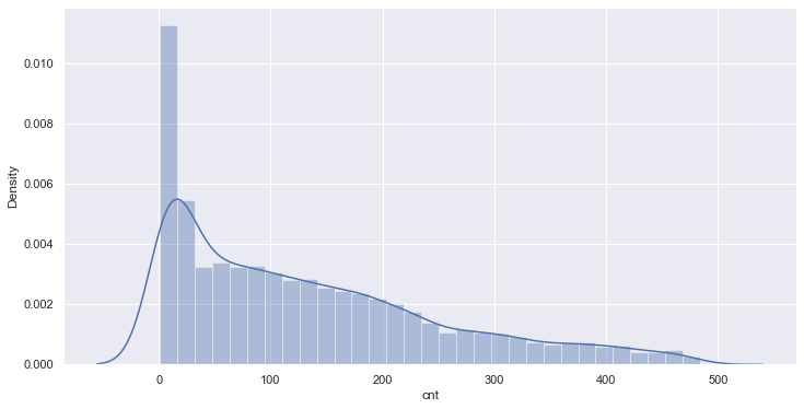
print("Training sample set without outliers: {}".format(len(train_preprocessed)))
sns.distplot(train_preprocessed.cnt);

Sample in train set with outliers: 10427
 Training sample set without outliers: 10151

correlation analysis

matrix = train[number_features + target].corr()
heat = np.array(matrix)
heat[np.tril_indices_from(heat)] = False
fig,ax= plt.subplots()
fig.set_size_inches(15,8)
sns.set(font_scale=1.0)
sns.heatmap(matrix, mask=heat,vmax=1.0, vmin=0.0, square=True,annot=True, cmap="Reds")

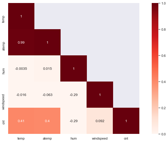
Conclusion: in descriptive analysis, the following points are summarized:

• The variables "Casual" and "registered" contain direct information about the shared bicycle count, and if this information is used for prediction (data leakage), they are not considered in the feature set.
• The variables "temp" and "atemp" are highly correlated. In order to reduce the dimension of the prediction model, the feature "atemp" can be deleted.
• The variables "hr" and "temp" seem to be the characteristics that make a greater contribution to predicting the number of bicycle sharing.

features.remove('atemp')

Overview of evaluation indicators

Mean Squared Error (MSE)

MSE = \sqrt{\frac{1}{N} \sum_{i=1}^N (x_i - y_i)^2}

Root Mean Squared Logarithmic Error (RMSLE)

RMSLE = \sqrt{ \frac{1}{N} \sum_{i=1}^N (\log(x_i) - \log(y_i))^2 }

R^2 Score

R^2=1-\frac{\sum_{i=1}^{n}e_i^2}{\sum_{i=1}^{n}(y_i-\bar{y})^2}

Model selection

The problems presented are characterized by:

• Regression: the target variable is a continuous value.
• Small data set: sample size less than 100K.
• A few features should be important: the correlation matrix indicates that a few features contain information to predict the target variable.

These characteristics give ridge regression, support vector regression, integrated regression, random forest regression and other methods a good opportunity to show their skills. For regression models, see previous articles.

Multicollinearity and ridge regression in linear regression Machine learning | simple and powerful detailed explanation of linear regression Machine learning | deep understanding Lasso regression analysis Master the support vector machine in sklearn Integrated algorithm random forest regression model Ten thousand words long text, deduce the strongest summary of eight linear regression algorithms! Principle + code, 11 regression models are summarized Basic mathematical principle of regression algorithm in machine learning

We will evaluate the performance of these models as follows:

x_train = train_preprocessed[features].values
y_train = train_preprocessed[target].values.ravel()
# Sort validation set for plots
val = val.sort_values(by=target)
x_val = val[features].values
y_val = val[target].values.ravel()
x_test = test[features].values

table = PrettyTable()
table.field_names = ["Model", 
                     "Mean Squared Error", 
                     "R² score"]

models = [
    SGDRegressor(max_iter=1000, tol=1e-3),
    Lasso(alpha=0.1),
    ElasticNet(random_state=0),
    Ridge(alpha=.5),
    SVR(gamma='auto', kernel='linear'),
    SVR(gamma='auto', kernel='rbf'),
    BaggingRegressor(),
    BaggingRegressor(KNeighborsClassifier(), 
                     max_samples=0.5, 
                     max_features=0.5),
    NuSVR(gamma='auto'),
    RandomForestRegressor(random_state=0, 
                          n_estimators=300)
]

for model in models: 
    model.fit(x_train, y_train) 
    y_res = model.predict(x_val)

    mse = mean_squared_error(y_val, y_res)
    score = model.score(x_val, y_val)    

    table.add_row([type(model).__name__, 
                  format(mse, '.2f'), 
                  format(score, '.2f')])

print(table)

+-----------------------+--------------------+----------+
|         Model         | Mean Squared Error | R² score |
+-----------------------+--------------------+----------+
|      SGDRegressor     |      43654.10      |   0.06   |
|         Lasso         |      43103.36      |   0.07   |
|       ElasticNet      |      54155.92      |  -0.17   |
|         Ridge         |      42963.88      |   0.07   |
|          SVR          |      50794.91      |  -0.09   |
|          SVR          |      41659.68      |   0.10   |
|    BaggingRegressor   |      18959.70      |   0.59   |
|    BaggingRegressor   |      52475.34      |  -0.13   |
|         NuSVR         |      41517.67      |   0.11   |
| RandomForestRegressor |      18949.93      |   0.59   |
+-----------------------+--------------------+----------+

Random forest

Stochastic forest model

The theory and practice of stochastic forest model can refer to the following two articles: Integrated algorithm random forest classification model Integrated algorithm random forest regression model

# Table setup
table = PrettyTable()
table.field_names = ["Model", "Dataset", "MSE", "MAE", 'RMSLE', "R² score"]
# model training
model = RandomForestRegressor(bootstrap=True, criterion='mse', max_depth=None,
           max_features='auto', max_leaf_nodes=None,
           min_impurity_decrease=0.0, min_impurity_split=None,
           min_samples_leaf=1, min_samples_split=4,
           min_weight_fraction_leaf=0.0, n_estimators=200, n_jobs=None,
           oob_score=False, random_state=None, verbose=0, warm_start=False)
model.fit(x_train, y_train) 

def evaluate(x, y, dataset): 
    pred = model.predict(x)
    mse = mean_squared_error(y, pred)
    mae = mean_absolute_error(y, pred)
    score = model.score(x, y)    
    rmsle = np.sqrt(mean_squared_log_error(y, pred))
    table.add_row([type(model).__name__, dataset,
                  format(mse, '.2f'), 
                  format(mae, '.2f'), 
                  format(rmsle, '.2f'), 
                  format(score, '.2f')])
    
evaluate(x_train, y_train, 'training')
evaluate(x_val, y_val, 'validation')

print(table)

+-----------------------+------------+----------+-------+-------+----------+
|         Model         |  Dataset   |   MSE    |  MAE  | RMSLE | R² score |
+-----------------------+------------+----------+-------+-------+----------+
| RandomForestRegressor |  training  |  298.21  | 10.93 |  0.21 |   0.98   |
| RandomForestRegressor | validation | 18967.46 | 96.43 |  0.47 |   0.59   |
+-----------------------+------------+----------+-------+-------+----------+

Characteristic importance

importances = model.feature_importances_
std = np.std([tree.feature_importances_ for tree in model.estimators_], axis=0)
indices = np.argsort(importances)[: : -1]

# Print out feature sorting
print("Feature ranking: ")

for f in range(x_val.shape[1]): 
    print("%d. feature %s (%f)" % (f + 1, features[indices[f]], importances[indices[f]]))

Feature ranking: 
1. feature hr (0.633655)
2. feature temp (0.160043)
3. feature hum (0.049495)
4. feature workingday (0.046797)
5. feature weathersit (0.027105)
6. feature windspeed (0.026471)
7. feature weekday (0.020293)
8. feature mnth (0.019940)
9. feature season (0.012995)
10. feature holiday (0.003206)

# Draw the characteristic importance of random forest
plt.figure(figsize=(14,5))
plt.title("Feature importances")
plt.bar(range(x_val.shape[1]), importances[indices], 
        color="cornflowerblue", yerr=std[indices], align="center")
plt.xticks(range(x_val.shape[1]), [features[i] for i in indices])
plt.xlim([-1, x_val.shape[1]])
plt.show())

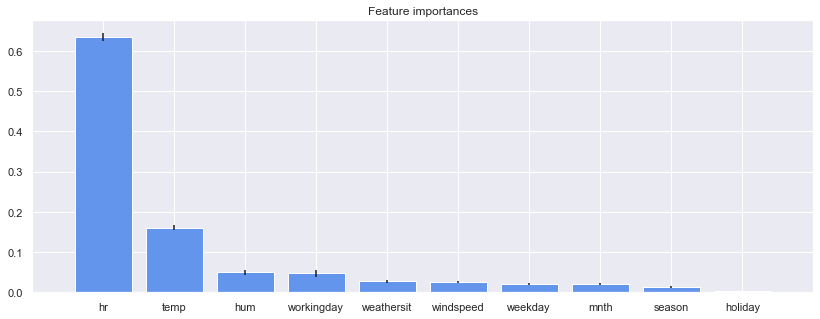
Analysis: the result corresponds to the high correlation between the variable "hour" and the variable "temperature" in the characteristic correlation matrix and the bicycle sharing count.

Write at the end

Here are some ideas to further improve the performance of the data model:

• Distribution adjustment of target variables: some prediction models assume that the distribution of target variables is normal distribution, and conversion in data preprocessing can improve the performance of these methods.
• Implementation of random forest for large-scale data sets. For large-scale data sets (> 10 Mio. Samples), if you can't save all samples in working memory, or you will encounter serious memory problems, it will be very slow to use python to implement the random forest in sklearn. One solution can be a woody implementation, which includes a top tree for pre classification and a flat random forest implemented in C language at the leaves of the top tree.