This is the first project I made with python. I also felt the power of python through this project. I randomly found two web pages containing a lot of data, both about solar flares. I will crawl the data of the two web pages together for analysis and sorting

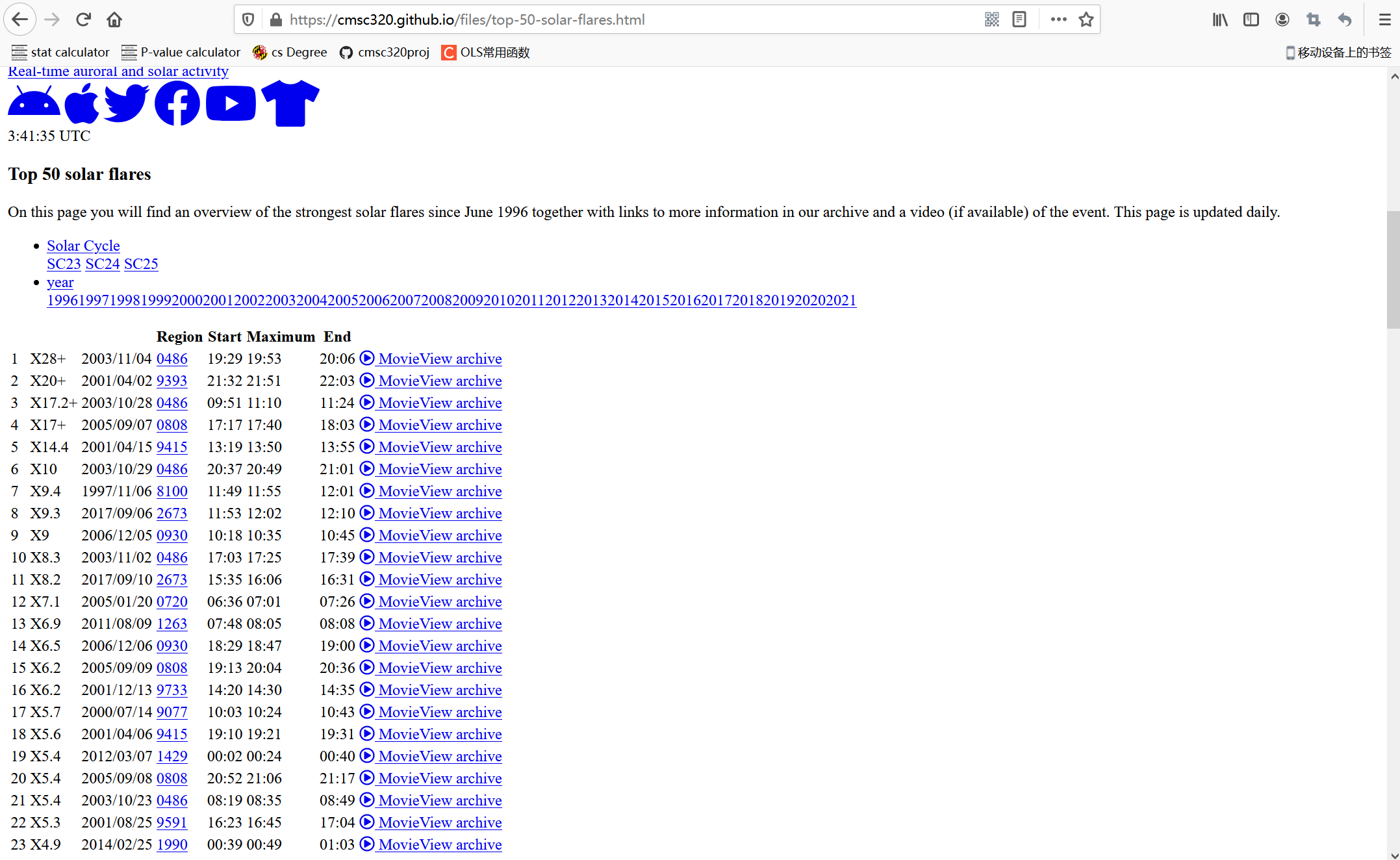
The website is: https://cmsc320.github.io/files/top-50-solar-flares.html

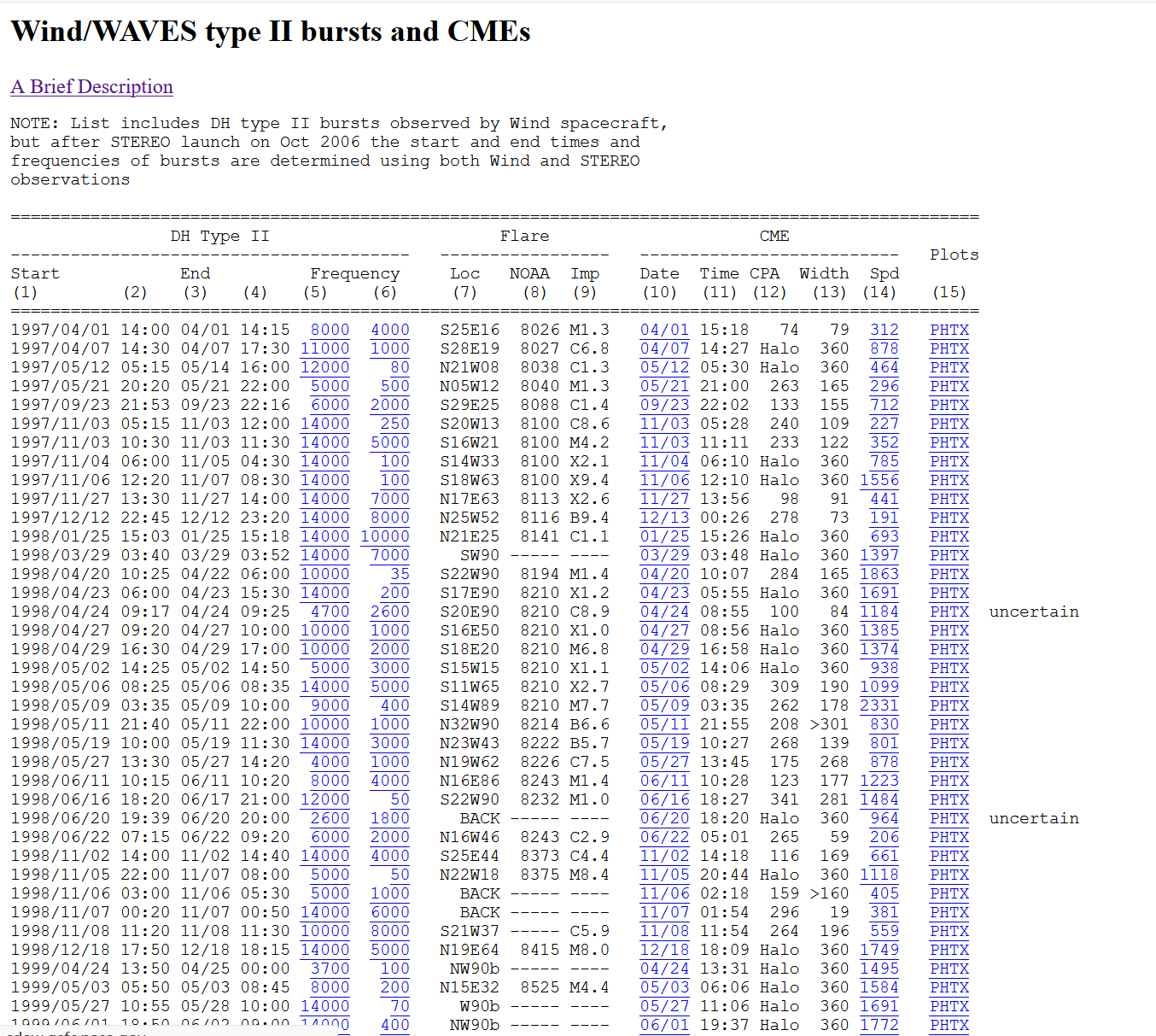
The URL of another page is: http://cdaw.gsfc.nasa.gov/CME_list/radio/waves_type2.html

The following is the general appearance of this web page. You can see that it displays the table of top50 solar flares. I will use python to crawl the data table of the modified web page and analyze it.

What another web page looks like

I used Google collab to write this project. The reason why I didn't choose vscode or docker to complete it is because I think collab is more convenient and powerful. When the code reports an error, there will be a shortcut key to directly jump to stackoverflow for query. Collab is a very powerful online compiler and is strongly recommended to write Jupiter book!

The following is the code for crawling data in the first part.

import requests
import pandas
import bs4
import numpy as np
import json
import copy

# step 1
# srcaping data from the website
response = requests.get('https://cmsc320.github.io/files/top-50-solar-flares.html')
soup = bs4.BeautifulSoup(response.text, features="html.parser")
soup.prettify()

# creating table
solar_table = soup.find('table').find('tbody')
data_table = pandas.DataFrame(columns=['rank', 'x_class', 'date', 'region', 'start_time', 'max_time', 'end_time', 'movie'], index = range(1,len(solar_table)+1))

# set data into table format
i = 0
for row in solar_table:
  k = 0
  columns = row.find_all('td')
  for col in columns:
    data_table.iat[i,k]=col.get_text()
    k += 1
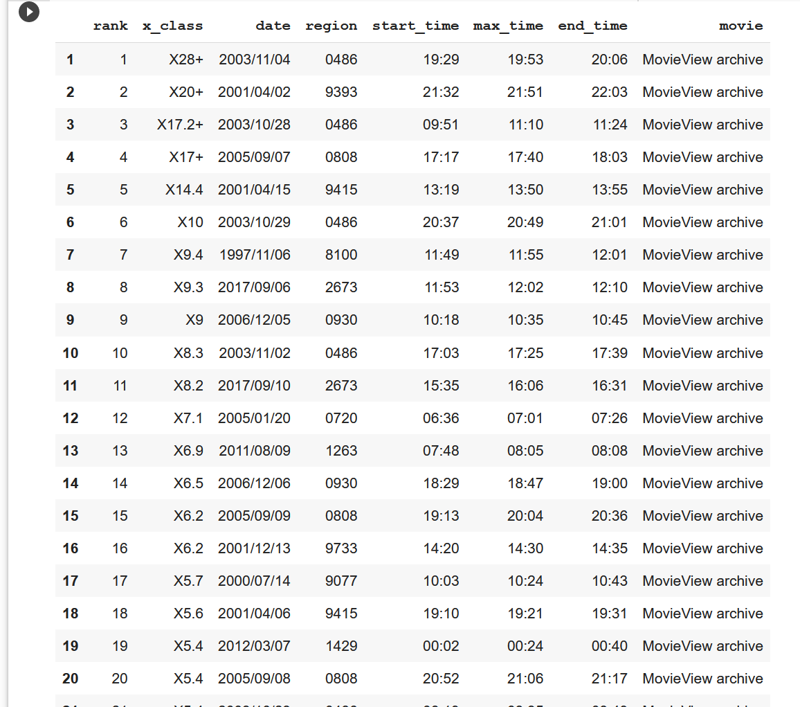
  i += 1

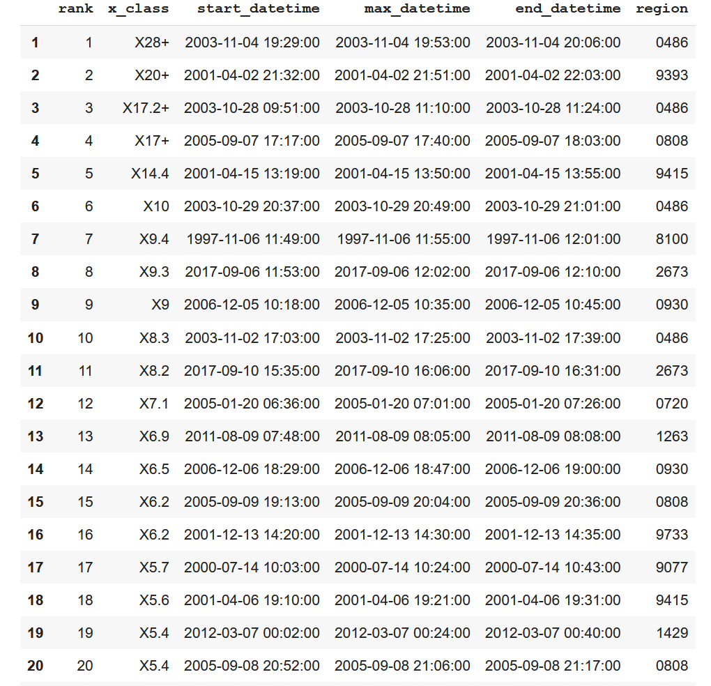
data_table

We can see that the actual 50 rows, that is, the table of the top flares in the first 50, are the same as the data on the web page and the corresponding data type.

Next, I will start data analysis. I will remove the last column of the generated table, and merge the date and the above three columns of data about the start time respectively, so that my table will become concise and data analysis later will be more convenient.

data_table = data_table.drop('movie', 1)

# Combine the date
start = pandas.to_datetime(data_table['date'] + ' ' + data_table['start_time'])
max = pandas.to_datetime(data_table['date'] + ' ' + data_table['max_time'])
end = pandas.to_datetime(data_table['date'] + ' ' + data_table['end_time'])

# Update values
data_table['start_datetime'] = start
data_table['max_datetime'] = max
data_table['end_datetime'] = end
data_table = data_table.drop('start_time', 1)
data_table = data_table.drop('max_time', 1)
data_table = data_table.drop('end_time', 1)
data_table = data_table.drop('date', 1)

# Set - as NaN
data_table = data_table.replace('-', 'NaN')
data_table = data_table[['rank', 'x_class', 'start_datetime', 'max_datetime', 'end_datetime', 'region']]

data_table

The adjusted table is as follows

In the third step, I will crawl the data of another web page mentioned above and save it into a new table

response2 = requests.get('https://cdaw.gsfc.nasa.gov/CME_list/radio/waves_type2.html')
soup2 = bs4.BeautifulSoup(response2.text, features="html.parser")
soup2.prettify()

# Creating data table
table2 = soup2.find('pre').get_text().splitlines()
del table2[0:12]
del table2[-1:]
data_table2 = pandas.DataFrame(columns = ['starting_date', 'starting_time', 'ending_date', 'ending_time', 'starting_frequency', 'ending_frequency', 
                        'solar_source', 'active_region', 'x-ray', 'date_of_CME', 'time_of_CME', 'position_angle', 'CME_width',
                        'CME_speed', 'plots'], index = range(1,len(table2)+1))

# Set data into the table
i = 0
for row in table2:
  table2[i] = (row.split('PHTX')[0] + 'PHTX').split()
  k = 0
  for col in table2[i]:
    data_table2.iat[i, k] = col
    k += 1
  i +=1

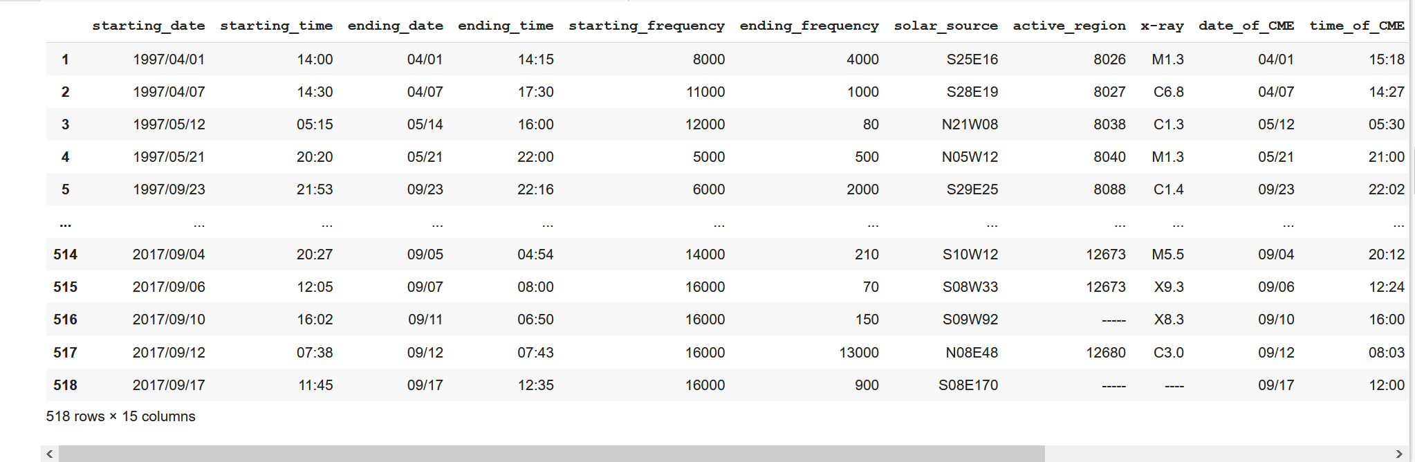
data_table2

The operation effect is as follows

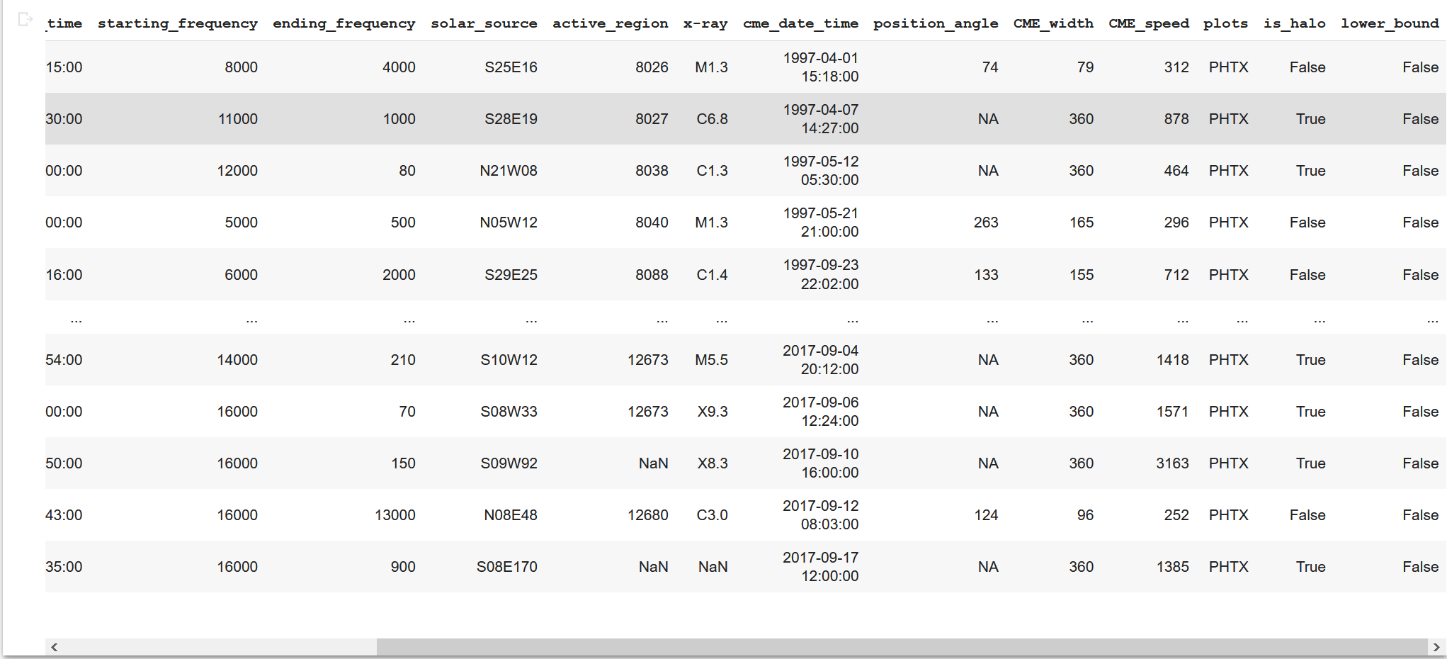
Next, I will sort out this new table, which I call NASA table. I will fill in NaN for the information in the missing position degree column, and then merge the date and time as above. I also created a new column to determine whether the width is lower bound

data_table2.replace(['----', '-----', '------', '--/--', '--:--', 'FILA', '????' 'LASCO DATA GAP', 'DSF'], 'NaN', inplace = True)

# Copy
data_table2['is_halo'] = data_table2['position_angle'].map(lambda x: x == 'Halo')
data_table2['position_angle'] = data_table2['position_angle'].replace('Halo', 'NA')
data_table2['lower_bound'] = data_table2['CME_width'].map(lambda x: x[0] == '>')
data_table2['CME_width'] = data_table2['CME_width'].replace('>', '')

# Set data in data_table2
for i, row in data_table2.iterrows():
  x = row['starting_date'][:5]
  data_table2.loc[i, 'starting_date'] = pandas.to_datetime(row['starting_date'] + ' ' + row['starting_time'])
  if row['ending_date'] != 'NaN' and row['ending_time'] !='NaN':
    if row['ending_time'] == '24:00':
      row['ending_time'] = '23:55'
    data_table2.loc[i, 'ending_date'] = pandas.to_datetime(x + row['ending_date'] + ' ' + row['ending_time'])
  if row['date_of_CME'] != 'NaN' and row['time_of_CME'] != 'NaN':
    data_table2.loc[i, 'date_of_CME'] = pandas.to_datetime(x + row['date_of_CME'] + ' ' + row['time_of_CME'])


data_table2 = data_table2.drop(['starting_time'], 1)
data_table2 = data_table2.drop(['ending_time'], 1)
data_table2 = data_table2.drop(['time_of_CME'], 1)
data_table2.rename(columns = {'starting_date':'starting_date_time', 'ending_date':'ending_date_time', 'date_of_CME':'cme_date_time'}, inplace=True)

data_table2

The sorted table is like this

Next, assist the first 50 lines from NASA table, and then build a new table

temp = data_table2.copy()

# Classifying only X leading
top_lines = temp.loc[temp['x-ray'].astype(str).str.contains('X')].copy()
top_lines['x-ray'] = top_lines['x-ray'].str.replace("X", '')
top_lines['x-ray'] = top_lines['x-ray'].astype(float)
top_lines = top_lines.sort_values('x-ray', ascending = False)
top_lines['x-ray'] = top_lines['x-ray'].astype(str)
top_lines['x-ray'] = 'X' + top_lines['x-ray']
top_lines = top_lines[0:50]
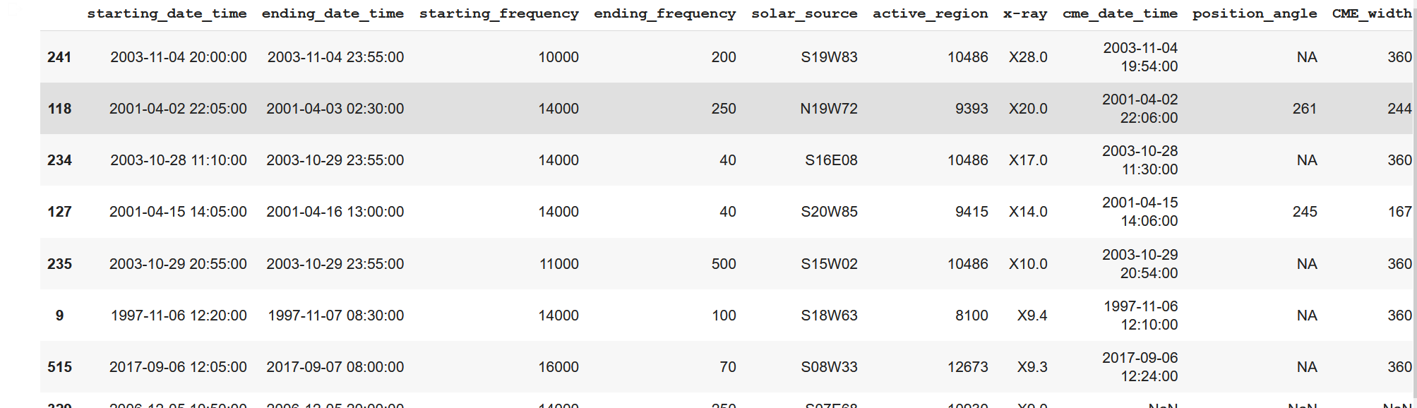
top_lines

As a result, the screenshot is not complete, but it can be seen that the top 50 of NASA table has been resurfaced

For the top 50 solar flares in the data of the first page, find the most matching row from the data of this new table.

top_lines['ranking'] = 'NA'

for i, i1 in data_table.iterrows():
  for j, j2 in top_lines.iterrows():
    if i1['region'] == j2['active_region'] and i1['start_datetime'].date() == j2['starting_date_time'].date():
      top_lines.loc[j, 'ranking'] = i

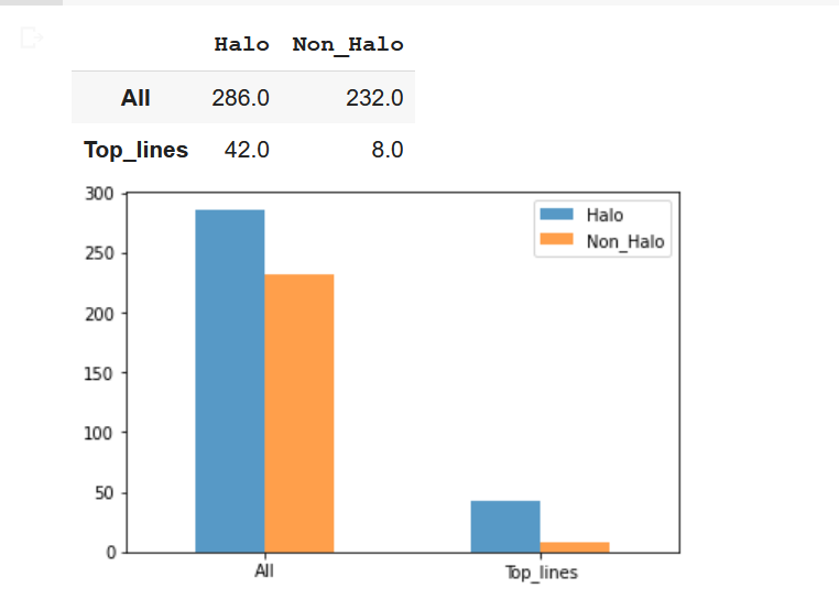
top_lines

Finally, I will analyze the data. I will draw a histogram to show the analysis results of the changes of a large number of attributes (start or end frequency, flare height or width) in the NASA table dataset over time.

halo_CME_top_lines = top_lines.is_halo.value_counts('True')[1] * len(top_lines.index)
non_halo_top_lines = len(top_lines.index) - halo_CME_top_lines
halo_nasa = data_table2.is_halo.value_counts('True')[1] * len(data_table2.index)
non_halo_nasa = len(data_table2.index) - halo_nasa

# Draw the graph
plot_graph = pandas.DataFrame({'Halo': [halo_nasa, halo_CME_top_lines], 'Non_Halo':[non_halo_nasa, non_halo_top_lines]}, index=['All', 'Top_lines'])
plot_graph.plot(kind = 'bar', alpha = 0.75, rot = 0)
plot_graph

Operation results