Let's practice, using the convolution basis of VGG16 network trained on ImageNet to extract interesting features from cat and dog images, and then train a cat and dog classifier on these features. VGG16 and other models are built into Keras. You can import from the Keras. Applications module. The following are some image classification models in keras.applications (all pre trained on ImageNet dataset):

• Xception
• Inception V3
• ResNet50
• VGG16
• VGG19
• MobileNet

We instantiate the VGG16 model.

1. Instantiate VGG16 convolution basis

from tensorflow.keras.applications import VGG16

conv_base = VGG16(weights='imagenet',
                  include_top=False,
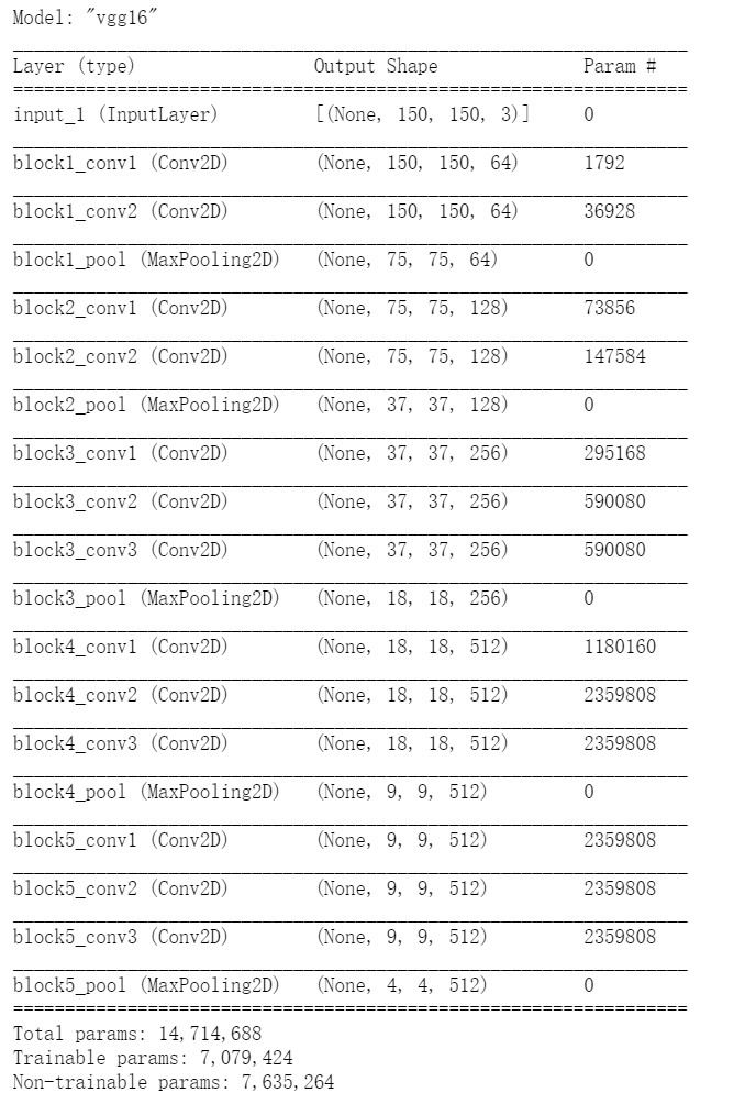
                  input_shape=(150, 150, 3))

conv_base.summary() #Detailed architecture of VGG convolution basis

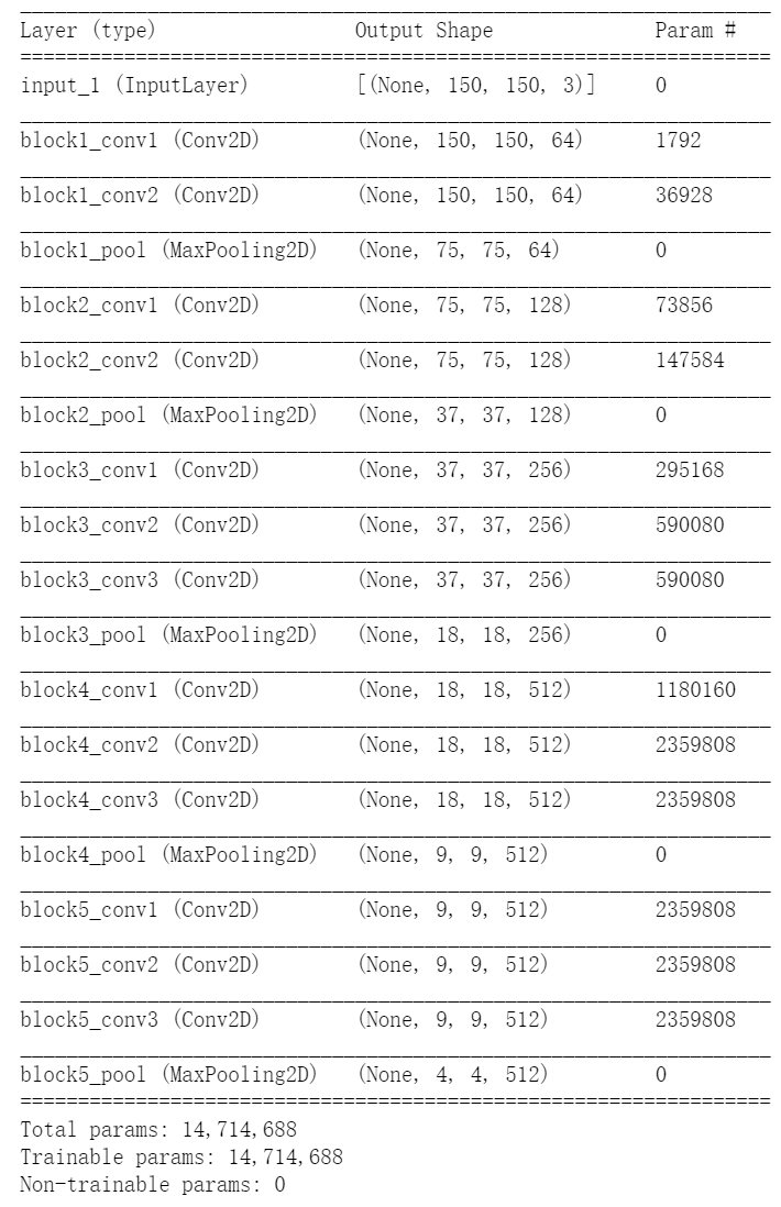
The final feature graph shape is (4, 4, 512). We will add a dense connection classifier to this feature. Next, there are two options for the next step.

• Run the convolution basis on your data set, save the output as a Numpy array on the hard disk, and then use this data as input to an independent dense connection classifier (similar to the classifier introduced in the first part of this book). This method has high speed and low computational cost, because it only needs to run the convolution basis once for each input image, and the convolution basis is the most expensive in the current process. But for the same reason, this approach does not allow you to use data enhancement.
• Add a sense layer at the top to extend the existing model (i.e. conv_base) and run the whole model end-to-end on the input data. In this way, you can use data enhancement because each input image will pass through the convolution basis when it enters the model. But for the same reason, the computational cost of this method is much higher than that of the first method.

2. Method 1: ① save your data in conv_base, and then use these outputs as inputs for the new model.

import os
import numpy as np
from keras.preprocessing.image import ImageDataGenerator

base_dir = 'D:\\Kaggle\\dogs-vs-cats-small'

train_dir = os.path.join(base_dir, 'train')
validation_dir = os.path.join(base_dir, 'validation')
test_dir = os.path.join(base_dir, 'test')

datagen = ImageDataGenerator(rescale=1./255)
batch_size = 20

def extract_features(directory, sample_count):
    features = np.zeros(shape=(sample_count, 4, 4, 512))
    labels = np.zeros(shape=(sample_count))
    generator = datagen.flow_from_directory(
        directory,
        target_size=(150, 150),
        batch_size=batch_size,
        class_mode='binary')
    i = 0
    for inputs_batch, labels_batch in generator:
        features_batch = conv_base.predict(inputs_batch)
        features[i * batch_size : (i + 1) * batch_size] = features_batch
        labels[i * batch_size : (i + 1) * batch_size] = labels_batch
        i += 1
        if i * batch_size >= sample_count:
            # Note that since generators yield data indefinitely in a loop,
            # we must `break` after every image has been seen once.
            #Note that these generators constantly generate data in the loop, so you must terminate the loop after reading all the images
            break
    return features, labels

train_features, train_labels = extract_features(train_dir, 2000)
validation_features, validation_labels = extract_features(validation_dir, 1000)
test_features, test_labels = extract_features(test_dir, 1000)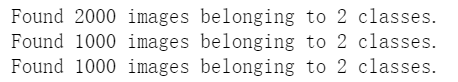

  At present, the extracted feature shapes are (samples, 4, 4, 512). We need to input it into the dense connection classifier, so we must flatten its shape to (samples, 8192) first.

#We need to input it into the dense connection classifier, so we must flatten its shape to (samples, 8192) first
train_features = np.reshape(train_features, (2000, 4 * 4 * 512))
validation_features = np.reshape(validation_features, (1000, 4 * 4 * 512))
test_features = np.reshape(test_features, (1000, 4 * 4 * 512))

Now you can define your dense connection classifier (note to use dropout regularization) and train the classifier on the data and tags just saved.

Method 1: ② define and train dense join classifiers

from keras import models
from keras import layers
from keras import optimizers
​
model = models.Sequential()
model.add(layers.Dense(256, activation='relu', input_dim=4 * 4 * 512))
model.add(layers.Dropout(0.5))
model.add(layers.Dense(1, activation='sigmoid'))
​
model.compile(optimizer=optimizers.RMSprop(lr=2e-5),
              loss='binary_crossentropy',
              metrics=['acc'])
​
history = model.fit(train_features, train_labels,
                    epochs=30,
                    batch_size=20,
                    validation_data=(validation_features, validation_labels))

Method 1: ③ draw the results

import matplotlib.pyplot as plt

acc = history.history['acc']
val_acc = history.history['val_acc']
loss = history.history['loss']
val_loss = history.history['val_loss']

epochs = range(1,len(acc)+1)

plt.plot(epochs, acc, 'bo', label='Training acc')
plt.plot(epochs, val_acc, 'b', label='Validation acc')
plt.title('Training and validation accuracy')
plt.legend()

plt.figure()

plt.plot(epochs, loss, 'bo', label='Training loss')
plt.plot(epochs, val_loss, 'b', label='Validation loss')
plt.title('Training and validation loss')
plt.legend()

plt.show()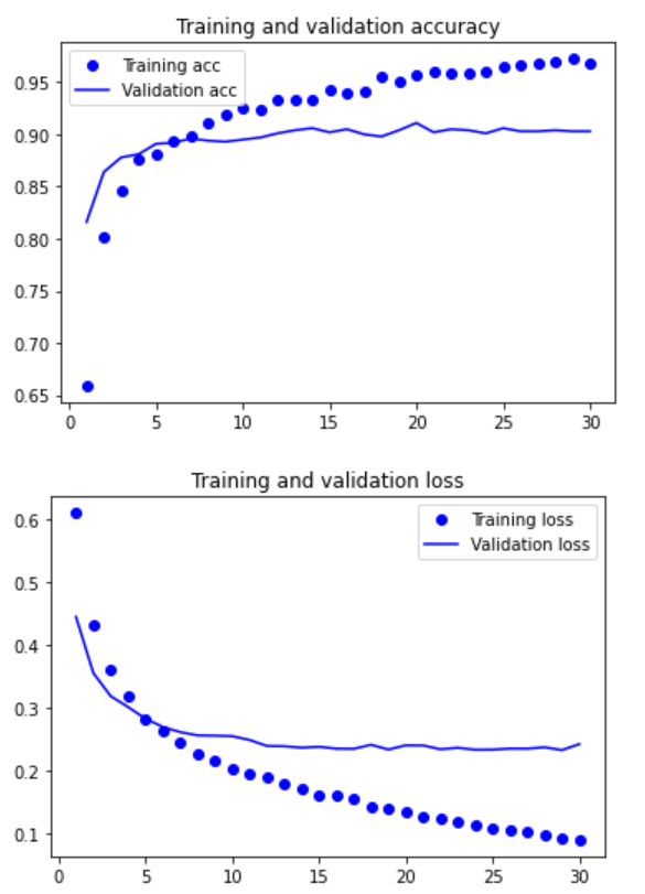

          Our verification accuracy is about 90%, which is much better than the small model trained from scratch in the previous section. However, it can also be seen from the figure that although the dropout ratio is quite large, the model has been fitted almost from the beginning. This is because this method does not use data enhancement, which is very important to prevent over fitting of small image data sets.

         Let's take a look at the second method of feature extraction, which is slower and more expensive, but data enhancement can be used during training. This method is to extend conv_base model, and then run the model end-to-end on the input data.

  3. Method 2: ① add a dense link classifier on the convolution basis.

from tensorflow.keras import models
from tensorflow.keras import layers

model = models.Sequential()
model.add(conv_base)
model.add(layers.Flatten())
model.add(layers.Dense(256, activation='relu'))
model.add(layers.Dense(1, activation='sigmoid'))

 

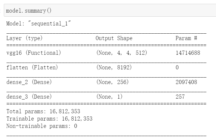
As you can see, the convolution basis of VGG16 has 14714688 parameters, very many. The classifier added to it has 2 million parameters.

The convolution basis must be "frozen" before compiling and training the model. freeze one or more layers means to keep their weights unchanged during training. If this is not done, the previously learned representation of the convolution basis will be modified during the training process. Because the density layer added on it is randomly initialized, very large weight updates will spread in the network, causing great damage to the previously learned representation.

In Keras, the way to freeze the network is to set its trainable property to False.

Method 2: ② freeze convolution basis

print('This is the number of trainable weights '
      'before freezing the conv base:', len(model.trainable_weights))

conv_base.trainable = False

print('This is the number of trainable weights '
      'after freezing the conv base:', len(model.trainable_weights))

          After this setting, only the weights of the two density layers added will be trained. There are four weight tensors in total, two in each layer (sovereign weight matrix and bias vector). Note that for these changes to take effect, you must first compile the model. If the trainable attribute of the weight is modified after compilation, the model should be recompiled, otherwise these modifications will be ignored.

         Now you can start training the model, using the same data enhancement settings as in the previous example.

Method 2: ③ using frozen convolution base to end training model

from tensorflow.keras.preprocessing.image import ImageDataGenerator

train_datagen = ImageDataGenerator(
      rescale=1./255,
      rotation_range=40,
      width_shift_range=0.2,
      height_shift_range=0.2,
      shear_range=0.2,
      zoom_range=0.2,
      horizontal_flip=True,
      fill_mode='nearest')

# Note that the validation data should not be augmented!
# Note that validation data cannot be enhanced
test_datagen = ImageDataGenerator(rescale=1./255)

train_generator = train_datagen.flow_from_directory(
        # This is the target directory
        train_dir,
        # All images will be resized to 150x150 × 150)
        target_size=(150, 150),
        batch_size=20,
        # Since we use binary_crossentropy loss, we need binary labels
#         Because binary is used_ Crossintropy is lost, so you need to use binary tags
        class_mode='binary')

validation_generator = test_datagen.flow_from_directory(
        validation_dir,
        target_size=(150, 150),
        batch_size=20,
        class_mode='binary')

model.compile(loss='binary_crossentropy',
              optimizer=optimizers.RMSprop(learning_rate=2e-5),
              metrics=['acc'])

history = model.fit_generator(
      train_generator,
      steps_per_epoch=100,
      epochs=30,
      validation_data=validation_generator,
      validation_steps=50,
      verbose=2)

It runs quite slowly

Method 2: ④ save the model

model.save('cats_and_dogs_small_3.h5')

Method 2: ⑤ draw the results

acc = history.history['acc']
val_acc = history.history['val_acc']
loss = history.history['loss']
val_loss = history.history['val_loss']
​
epochs = range(len(acc))
​
plt.plot(epochs, acc, 'bo', label='Training acc')
plt.plot(epochs, val_acc, 'b', label='Validation acc')
plt.title('Training and validation accuracy')
plt.legend()
​
plt.figure()
​
plt.plot(epochs, loss, 'bo', label='Training loss')
plt.plot(epochs, val_loss, 'b', label='Validation loss')
plt.title('Training and validation loss')
plt.legend()
​
plt.show()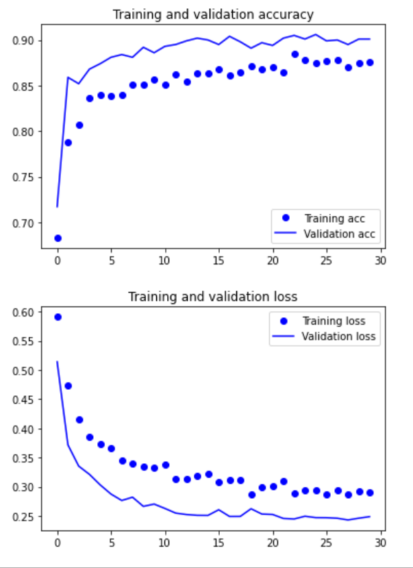

 

Let's draw the results again. As you can see, the verification accuracy is about 96%. This is much better than the small convolutional neural network trained from scratch.

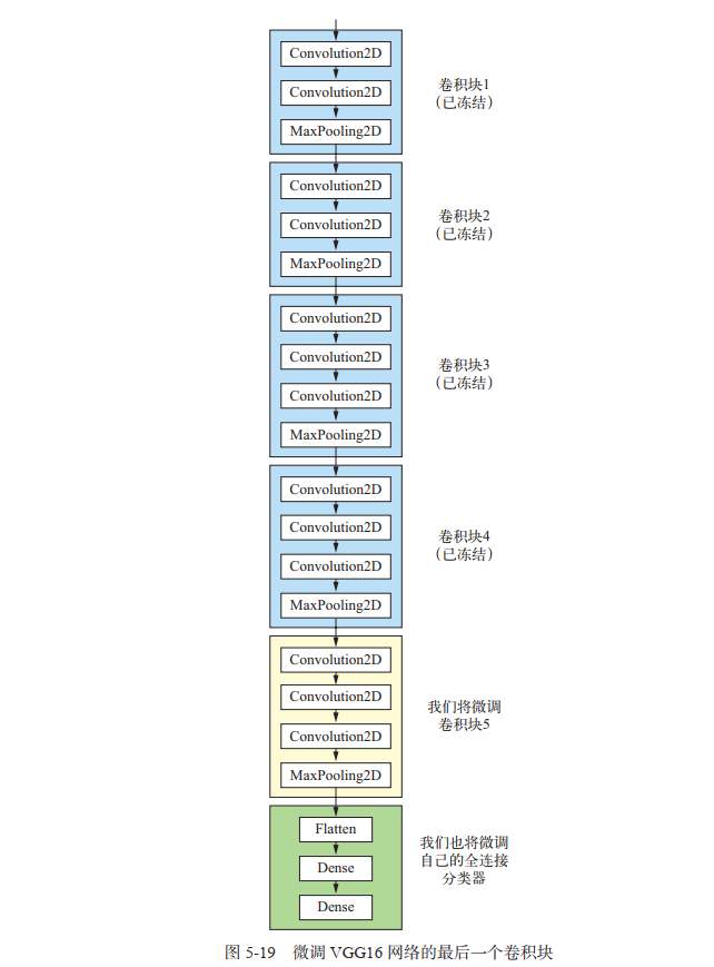
Fine tuning model

Another widely used model reuse method is fine tuning, which is complementary to feature extraction. For the frozen model base used for feature extraction, fine tuning refers to "thawing" the top layers, and jointly training the thawed layers with the newly added part (in this case, the fully connected classifier) (see the figure below). It is called fine tuning because it only slightly adjusts the more abstract representations in the reused model to make them more relevant to the problem at hand.

 

As mentioned earlier, the convolution basis of VGG16 is frozen to train a randomly initialized classifier. Similarly, only when the above classifier has been trained can the top layers of convolution basis be fine tuned. If the classifier is not well trained, the error signal transmitted through the network during training will be particularly large, and the representations learned before the fine-tuning layers will be destroyed. Therefore, the steps to fine tune the network are as follows.

• (1) Add a custom network to the trained base network.
• (2) Freeze the base network.
• (3) The part added to the training.
• (4) Thaw some layers of the base network.
• (5) Joint training thawed these layers and added parts. You have completed the first three steps in feature extraction. Let's continue with step 4: thaw the conv first_ Base, and then freeze some of the layers.

Remind me, the architecture of convolution basis is as follows.

   4. Freeze all layers up to a layer

conv_base.trainable = True

set_trainable = False
for layer in conv_base.layers:
    if layer.name == 'block5_conv1':
        set_trainable = True
    if set_trainable:
        layer.trainable = True
    else:
        layer.trainable = False

5. Fine tune the model

model.compile(loss='binary_crossentropy',
              optimizer=optimizers.RMSprop(learning_rate=1e-5),
              metrics=['acc'])

history = model.fit_generator(
      train_generator,
      steps_per_epoch=100,
      epochs=100,
      validation_data=validation_generator,
      validation_steps=50)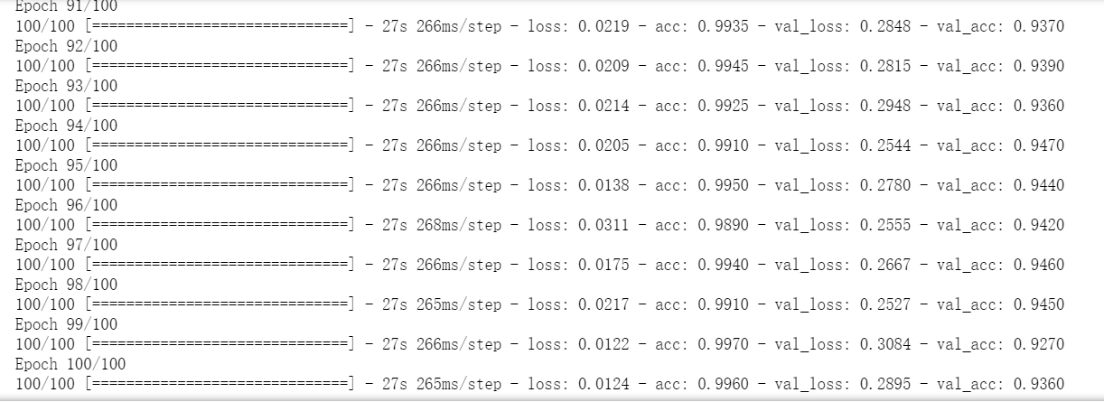

 

 

The operation is quite slow: 40min!  

#Save model
model.save('cats_and_dogs_small_4.h5')

#Draw results
acc = history.history['acc']
val_acc = history.history['val_acc']
loss = history.history['loss']
val_loss = history.history['val_loss']

epochs = range(len(acc))

plt.plot(epochs, acc, 'bo', label='Training acc')
plt.plot(epochs, val_acc, 'b', label='Validation acc')
plt.title('Training and validation accuracy')
plt.legend()

plt.figure()

plt.plot(epochs, loss, 'bo', label='Training loss')
plt.plot(epochs, val_loss, 'b', label='Validation loss')
plt.title('Training and validation loss')
plt.legend()

plt.show()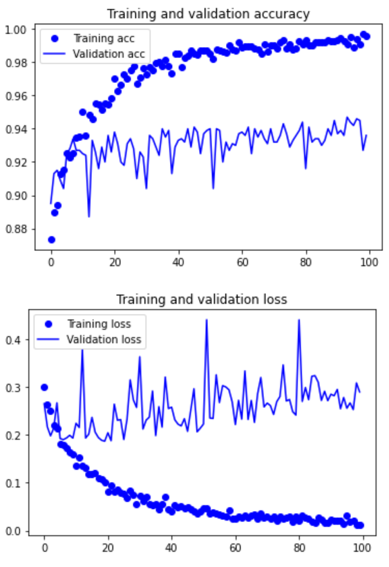

These curves appear to contain noise. To make the image more readable, you can replace each loss and accuracy with an exponential moving average to smooth the curve. The following is a simple practical function  :

  7. Make the curve smooth

def smooth_curve(points, factor=0.8):
  smoothed_points = []
  for point in points:
    if smoothed_points:
      previous = smoothed_points[-1]
      smoothed_points.append(previous * factor + point * (1 - factor))
    else:
      smoothed_points.append(point)
  return smoothed_points

plt.plot(epochs,
         smooth_curve(acc), 'bo', label='Smoothed training acc')
plt.plot(epochs,
         smooth_curve(val_acc), 'b', label='Smoothed validation acc')
plt.title('Training and validation accuracy')
plt.legend()

plt.figure()

plt.plot(epochs,
         smooth_curve(loss), 'bo', label='Smoothed training loss')
plt.plot(epochs,
         smooth_curve(val_loss), 'b', label='Smoothed validation loss')
plt.title('Training and validation loss')
plt.legend()

plt.show()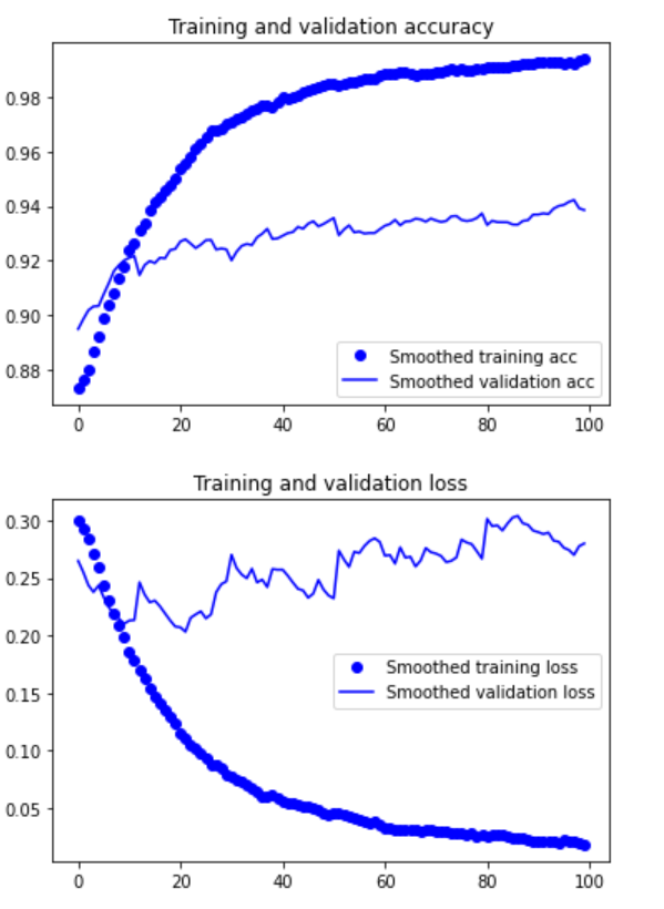

Verify that the accuracy curve becomes clearer. It can be seen that the accuracy value is increased by 1%, from about 96% to more than 97%.

Note that there is no real improvement (actually getting worse) from the loss curve. You may wonder, if the loss is not reduced, how can the accuracy remain stable or improve? The answer is simple: the figure shows the average value of pointwise loss value, but the distribution of loss value rather than the average value affects the accuracy, because the accuracy is the binary threshold of category probability predicted by the model. Even if it cannot be seen from the average loss, the model may still be improving.

Now, you can finally evaluate the model on the test data.

 

  8. Finally evaluate the model on the test data

test_generator = test_datagen.flow_from_directory(
        test_dir,
        target_size=(150, 150),
        batch_size=20,
        class_mode='binary')

test_loss, test_acc = model.evaluate_generator(test_generator, steps=50)
print('test acc:', test_acc)

  

Summary

Here are the main points you should learn from the exercises in the above two sections.

• Convolutional neural network is the best machine learning model for computer vision tasks. A convolutional neural network can be trained from scratch even on a very small data set, and the results are good.
• The main problem on small data sets is over fitting. When processing image data, data enhancement is a powerful method to reduce over fitting.
• Using feature extraction, the existing convolutional neural network can be easily reused in new data sets. This is a valuable method for small image data sets.
• As a supplement to feature extraction, you can also use fine tuning to apply some data representations previously learned from existing models to new problems. This method can further improve the performance of the model.

Now you have a set of reliable tools to deal with image classification problems, especially for small data sets.