What is computer science?
● first of all, it is clear that computer science is not only the research of computer. Although computer has played an important role in the process of scientific development, it is only a tool, a tool without soul. The so-called computer science is actually the research on problems, solving problems and solutions produced in the process of solving problems. For example, given a problem, the goal of computer scientists is to develop an algorithm to deal with the problem, and finally get the solution or optimal solution of the problem. Therefore, computer science can also be regarded as the study of algorithms. Therefore, we can also feel that the so-called algorithm is an implementation idea or idea to deal with and solve the problem.
How to visualize the understanding algorithm
● an ever victorious general will formulate strategies before fighting, in order to win the final victory in the shortest time and at the lowest cost. If coding is used as a battlefield, the programmer is the commander of the battle. How can you get the final execution result of your program in the shortest time and with the least resource consumption? Algorithm is our strategy!
Methods of judging the advantages and disadvantages of procedures
● consumption of computer resources and execution efficiency (not recommended, not intuitive)
● time consuming calculation algorithm execution (properly recommended, because it will be affected by the machine and execution environment)
● time complexity (recommended)
Time complexity
● evaluation rules: quantify the number of operations / steps performed by the algorithm
● most important item: the most meaningful item in the time complexity expression
● Big O notation: it is the expression of measuring the quality of the algorithm by time complexity.
■ o (the most important)
def sumOfN(n):
    theSum = 0 #1
    for i in range(1,n+1):
        theSum = theSum + i #n
    return theSum Office 1
    print ( sumOfN(10))
# Time complexity n+1+1
# O(n)
a=5
b=6
c=10
for i in range(n):
for j in range(n) :
x = i * i
y = j * j
z = i * j
for k in range(n):
w=a*k+45
v=b*b
d=33
# Time complexity 3 + 3n**2 + 2n + 1
# O(n**2)● common time complexity:
■0(1)< O( ) < 0(n) < O(n) < 0(n^2) < 0(n^3) < 0(2^n) < O(n) < o(n^n)
data structure
● concept: the organization of data (basic types of data (intg,float,char)) is called data structure. The data structure solves how to save a group of data and how to save it.
● different forms are used to organize data, and the time complexity based on query is different. Therefore, it is considered that the algorithm is designed to solve practical problems, and the data structure is the carrier of the problem that the algorithm needs to deal with.
Performance analysis of python structure
● instantiate an empty list, and then add the data in the range of 0-n to the list. (four methods)
● timeit module: This module can be used to test the execution speed / duration of a piece of python code.
● Timer class: this class is specially used in the timeit module to measure the execution speed and duration of python code. Prototype: Class
timeit.Timer(stmt=' 'pass',setup='pass').
■ stmt parameter: indicates the code block statement to be tested.
■ setup: the settings required to run code block statements.
● timeit function: timeit Timer. timeit(number10000),. This function returns the average time taken to execute a code block statement number times.
from timeit import Timer
def test01():
    alist=[]
    for i in range(1000):
        alist.append(i)
    return alist
def test02():
    alist=[]
    for i in range(1000):
        alist = alist + [i]
    return alist
def test03():
    alist = [i for i in range(1000)]
    return alist
def test04():
    alist=list(range(1000))
    return alist
if__name__ == '__main__':
    timer = Timer(stmt='test01()',setup='from __main__ import test01')
Stack
● features: first in and last out
● stack top and bottom
■ add elements from the top of the stack to the bottom of the stack, and take elements from the top of the stack
● application: each web browser has a return button. When you browse web pages, they are placed in a stack (actually the web address of the page) The page you are viewing now is at the top, and the first page you are viewing is at the bottom. If you press the 'back' button, you will browse the previous pages in the reverse order.
● Stack() creates an empty new stack. It does not require parameters and returns an empty stack.
● push(item) adds a new item to the top of the stack. It requires item as a parameter and does not return anything.
● pop() deletes the top item from the stack. It does not require parameters and returns item The stack has been modified.
● peek() returns the top item from the stack, but does not delete it. No parameters are required. Do not modify the stack.
● isEmpty() tests whether the stack is empty. No arguments are required and a Boolean value is returned
● size() returns the number of item s in the stack. No parameters are required and an integer is returned.
class Stack():
    def __init__(self):#Build an empty stack
        self.items=[]
    def push(self,item):
        #Add from top to bottom
        self.items.append(item)
    def pop(self):
        #Take elements from the top of the stack to the bottom of the stack
        return self.items.pop()
    def peek(self):#Returns the subscript of the stack top element
        return len(self.items)-1
    def isEmpty(self):
        return self.items == [ ]
    def size(self):
        return len(self.items)
Queue ● queue: first in first out
● application scenario:
■ our computer lab has 30 computers connected to a printer. When students want to print, their print task is "consistent" with all other print tasks they are waiting for. The first entry task is to complete it first. If you are the last one, you must wait for all other tasks in front of you to print
● Queue() creates an empty new queue. It does not require parameters and returns - an empty queue.
● enqueue(item) adds a new item to the end of the queue. It requires iterm as a parameter and does not return anything.
● dequeue() removes items from the head of the queue. It does not require parameters and returns item The queue was modified.
● isEmpty() check whether the queue is empty It does not require parameters and returns a Boolean value
● size() returns the number of items in the queue. It does not require parameters and returns an integer.
class Queue():
    def __init__(self):#Build an empty stack
        self.items=[]
    def enqueue(self,item):
        #Add from top to bottom
        self.items.insert(0, item)
    def dequeue(self):
        #Take elements from the top of the stack to the bottom of the stack
        return self.items.pop()
    def isEmpty(self):
        return self.items == [ ]
    def size(self):
        return len(self.items)
Double ended queue
● compared with the same column, there are two heads and tails. It can insert and delete data at both ends, and provides the characteristics of stack and queue in single data structure
● Deque0 creates an empty new deque It does not require parameters and returns an empty deque
● addFront(tem) - adds a new item to the header of deque. It requires the item parameter and does not return anything.
● addrealitem) adds - new items to the tail of deque. It requires the item parameter and does not return anything.
● removeFront() deletes the first item from deque. It does not require parameters and returns item Deque was modified.
● removeRear0 delete the tail item from deque. It does not require parameters and returns item, and deque is modified.
● isEmpty0 test whether deque is empty It does not require parameters and returns a Boolean value.
● size0 returns the number of items in deque. It does not require parameters and returns - an integer.
Memory
● role of computer
■ storing and computing binary data.
● how does the computer realize 1 + 1 =? operation
■ load 1 into the computer memory, and then add the data stored in the specified memory based on the addition register of the computer.
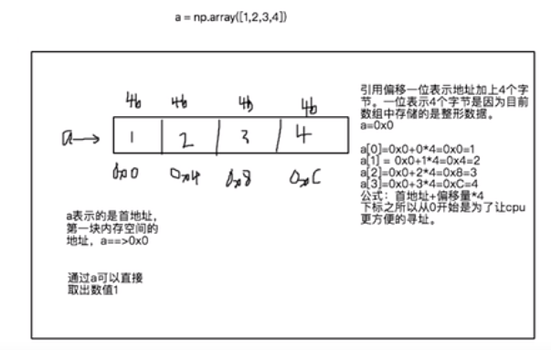
● concept of variables
■ essentially, a variable refers to a - block of memory space in a computer.
■ memory space has two inherent properties
. Address: expressed as a hexadecimal number
. Function: convenient cup addressing. House number.
. Size: bit, byte kb,. mb. gb. tb
. Determines the range of values stored in the block memory
● understand the memory diagram of a=10 (reference, pointing)
■ reference: it is a variable. Usually, the variable represents the address of a - block of memory space.
■ pointing: if a variable or reference stores an address representing a block of memory space, the variable or reference points to the block of memory space.
● memory space occupied by different data
■ bit: 1 bit can only store -- bit binary numbers.
■ byte: 8bit
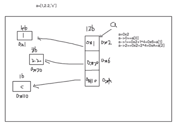
The difference between array and list. For the list, because the space opened up by the address is different, the data cannot be retrieved in sequence, so another continuous space is generated as the container for storing the address.
● disadvantages of sequence table: the structure of sequence table needs to know the data size in advance to apply for continuous storage space, and the data needs to be relocated during expansion.
Compared with sequential list, linked list structure can make full use of computer memory space, realize flexible memory dynamic management, and there is no need to move data during expansion.
● linked list is a common basic data structure. It is a linear table, but unlike sequential table, it continuously stores data, but each node (data storage unit) stores the information (i.e. address) of the next node
● is_empty(): whether the linked list is empty
● length(): the length of the linked list
● travel(): traverse the entire linked list
● add(item): add an element to the head of the linked list
● append(item): add an element at the end of the linked list
● insert(pos, item): add an element at a specified location
● remove(item): delete a node
● search(item): find whether the node exists
# Encapsulation of nodes
class Node():
    def __init__(self,item):
        self.item = item
        self.next = None
#Encapsulation of linked list
class Link():
    def __init__(self):#Build an empty linked list
        # Here is an address
        self._head = None
    # head always points to the first node in the linked list. None indicates that there is no node in the linked list.
    def add(self, item):
        node = Node(item)
        node.next = self._head
        self._head = node  # The node here is the address

    def travel(self):
        cur = self._head
        while cur:
            print(cur.item)
            cur = cur.next

    def isEmpty(self):
        return self._head == None

    def length(self):
        cur = self._head
        count = 0
        while cur:
            count += 1
            cur = cur.next
        return count

    def append(self, item):
        node = Node(item)
        # If the linked list is empty
        if self._head == None:
            self.add(item)
            self._head = node
            return
        # If the linked list is not empty
        pre = None  # pre refers to a node in front of cur
        cur = self._head
        while cur:
            pre = cur
            cur = cur.next
        pre.next = node
    # Query whether the item exists in the linked list
    def search(self, item):
        find = False
        cur = self._head
        while cur:
            if cur.item == item:
                find = True
                break
            else:
                cur = cur.next
        return find

    def insert(self, pos, item):
        node = Node(item)
        cur = self._head
        pre = None
        # Judge the case where the position is 0
        if pos == 0:
            self._head = node
            node.next = cur
        for i in range(pos):
            pre = cur
            cur =cur.next
        pre.next = node
        node.next = cur
    def remove(self, item):
        pre = None
        cur = self._head
        if self._head.item == item:
            self._head = cur.next
            return
        while cur:
            pre = cur
            cur = cur.next
            if cur.item == item:
                pre.next = cur.next
                return
    def reverse(self):
        pre = self._head
        cur = pre.next
        next_node = cur.next
        pre.next = None
        while True:
            cur.next = pre
            #pre,next,next_node backward offset
            pre = cur
            cur = next_node
            if next_node != None:
                next_node = next_node.next
            else:
                break
        self._head = pre
Binary tree
● root node: the upper node in the tree
● left leaf node
● right leaf node
● subtree
■ complete subtree
. A root node, consisting of left and right leaf nodes
■ incomplete subtree
. Root node, left leaf node
. Root node, right leaf node
. Root node
. Features: each node can be used as the root node of a -- subtree
class Node():
    def __init__(self, item):
        self.item = item
        self.left = None  # Point to the left leaf node of this node
        self.right = None  # Point to the right leaf node of this node
class Tree():
    def __init__(self):
        self.root = None # Always point to the root node in the binary tree
    # Top to bottom, left to right insertion
    def insert(self, item):
        node = Node(item)
        # If the tree is empty
        if self.root == None:
            self.root = node
            return
        # If not empty
        cur = self.root
        q = [cur]
        while True:
            n = q.pop(0)
            if n.left != None:
                q.append(n.left)
            else:
                n.left = node
                break
            if n.right != None:
                q.append(n.right)
            else:
                n.right = node
                break

    def travel(self):
        cur = self.root
        q = [cur]
        while q:
            n = q.pop(0)
            print(n.item)
            if n.left != None:
                q.append(n.left)
            if n.right != None:
                q.append(n.right)
    def forward(self, root):
        if root == None:
            return
        print(root.item)
        self.forward(root.left)
        self.forward(root.right)
    def middle(self, root):
        if root == None:
            return
        self.middle(root.left)
        print(root.item)
        self.middle(root.right)
    def back(self, root):
        if root == None:
            return
        self.back(root.left)
        self.back(root.right)
        print(root.item)
● implementation idea of depth traversal
■ depth traversal needs to be applied to each - subtree
■ the difference between subtree and subtree is reflected in the root node.
■ if you write a function that can traverse the nodes in a subtree, you can traverse the whole tree in depth by applying the function to other subtrees. (sort binary tree)
class SortTree():
    def __init__(self):
        self.root = None
    def add(self, item):  # Inserts a node into a sorted binary tree
        node = Node(item)
        if self.root == None: # When the tree is empty
            self.root = node
            return
        cur =self.root
        while True:
        # Tree is not empty
            if cur.item > item: #  The value of the inserted node is less than the root node, which needs to be inserted to the left of the root node
                if cur.left == None:
                    cur.left = node
                    break
                else:
                    cur = cur.left
            else: # The value of the inserted node is greater than the root node, which needs to be inserted to the right of the root node
                if cur.right == None:
                    cur.right = node
                    break
                else:
                    cur = cur.right
    def middle(self, root):
        if root == None:
            return
        self.middle(root.left)
        print(root.item)
        self.middle(root.right)
Binary search:
It is to perform binary search on the ordered list, compare half of the values, and then search up or down
Bubble sort:
Compare the numbers in pairs and put the big one behind. Gradually put the maximum value last. (double cycle)
● select sort
1. Compare the elements in the out of order sequence to find the maximum value, and then directly place the maximum value at the last position of the sequence (double-layer loop)
● insert sort
● ideas:
● the original sequence needs to be divided into two parts: ordered part and unordered part
■ insert the elements in the unordered part into the ordered part one by one. Note: initially, the ordered part is the first element of the unordered sequence, The disordered part is n-1 elements of the disordered sequence ■ disordered sequence: [3,8,5,7.6] 3 is the initial ordered part, and 8,5,7,6 is the initial disordered part
def sort(alist) :
    for i in range(1, len(alist)):
        while i > 0:
            if alist[i-1] > alist[i]:
                alist[i-1], alist[i] = alist[i], alist[i-1]
                i -= 1
            else:
                break
    return alist
● Hill sort
■ key variable: incremental gap
■ gap: the initial value is len(alist)//2
. 1. Indicates the number of groups grouped
. 2. Interval between each set of data
■ insertion sort is a hill sort with increment of 1
#  1. Add the concept of increment to the insertion sort code
def sort(alist) :
    gap = len(alist) // 2 # initial increment
    #The insert sort is a hill sort with an increment of 1
    #The increment of the following code is 1, and 1 in the following code represents increment
    """for i in range(1, len(alist)):
        while i > 0:
            if alist[i-1] > alist[i]:
                alist[i-1], alist[i] = alist[i], alist[i-1]
                i -= 1
            else:
                break"""
    #Replace increment 1 in the insertion sort with gap
    #From increment of 1 to increment of gap
    while gap >= 1:
        for i in range(gap, len(alist)):
            while i > 0:
                if alist[i-gap] > alist[i]:
                    alist[i-gap], alist[i] = alist[i], alist[i-gap]
                    i -= gap
                else:
                    break
        gap //= 2
    return alist
● quick sort
■ set the first element in the list as the reference number, assign it to the mid variable, and then set the value smaller than the reference in the whole list
Place on the left side of the datum and the number to which the datum is compared on the right side of the datum. Then the sequence on the left and right sides of the reference number is set according to this
Method for discharge.
■ define two pointers, low points to the leftmost and high points to the rightmost
■ then move the rightmost pointer to the left. The moving rule is that if the value pointed by the pointer is smaller than the reference, the pointer will be pointed to the left
Move the number to the original position of the reference number, otherwise continue to move the pointer.
■ if the value pointed by the rightmost pointer moves to the reference position, start moving the leftmost pointer and move it to the right, if
If the value pointed by the pointer is greater than the benchmark, move the value to the position pointed by the rightmost pointer, and then stop moving.
■ if the left and right pointers repeat, put the reference into the position where the left and right pointers repeat, the left side of the reference is a smaller value than it, and the right side is a smaller value
Side is a larger value.
def firstSort(alist, left, right):#1. Core operation: place the cardinality mid in the middle of the sequence so that the left side of the cardinality is smaller than it and the right side is larger than it
# eft and right indicate which - subsequence the current sort recursion acts on
    low = left  # First element subscript
    high = right  # Last element subscript
    if low > high:
        return

    mid = alist[low]  # base
    while low != high:
        while low < high:
            if mid <= alist[high]:  # To offset 1 to the left, there must be equal to, otherwise when there are the same elements, the loop will not jump out, the same below, otherwise the exit condition will have to be changed
                high -= 1
            else:
                alist[low] = alist[high]
                break
        while low < high:
            if mid >= alist[low]:
                low += 1
            else:
                alist[high] = alist[low]
                break
    alist[low] = mid
    #The above is the core operation, which needs to be recursive into the left and right subsequences
    firstSort(alist, left, low-1) #Apply sort to the left sequence
    firstSort(alist, high+1, right) #Apply sort to the right sequence
    return alist