1, Algorithm Introduction
Linear regression: supervised learning ---- > regression algorithm
2, Algorithm principle
Linear regression is an analytical method that uses regression equation (function) to model the relationship between one or more independent variables (eigenvalues) and dependent variables (target values)
General formula:
 Loss function:
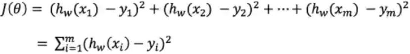 yi is the true value of the ith training sample
h(xi) is the characteristic value combination prediction function of the ith training sample
Also known as least square method
Normal equation:
 x is the eigenvalue matrix and y is the target value matrix. Get the best result directly
3, Univariate linear regression
1. Simple
import numpy as np
import matplotlib.pyplot as plt

# The regression equation is established as follows: y = kx + b is a univariate regression equation

X = np.array([[150],
              [200],
              [250],
              [300],
              [350],
              [400],
              [600]
              ])

X = X.reshape(-1, )

y = np.array([6450, 7450, 8450, 9450, 11450, 15450, 18450])

m = len(y)

x_mean = np.mean(X)  # Mean value of x
fenzi = np.sum(y * (X - x_mean))

fenmu = np.sum(X ** 2) - 1 / m * (np.sum(X) ** 2)
w = fenzi / fenmu

b = 1 / m * np.sum((y - w * X))

print("Coefficient and intercept", w, b)

# y = 28.77659574468084 + 1771.8085106383014

y_pred = X * w + b
plt.scatter(X, y)
plt.plot(X, y_pred)
plt.show()
2,sklearn
from sklearn.linear_model import LinearRegression
import numpy as np
import matplotlib.pyplot as plt


X = np.array([[150],
              [200],
              [250],
              [300],
              [350],
              [400],
              [600]
              ])

y = np.array([6450, 7450, 8450, 9450, 11450, 15450, 18450])

# instantiation
lr = LinearRegression()

lr.fit(X, y)

print("Coefficient and intercept", lr.coef_[0], lr.intercept_)

y_pred = lr.predict(X)

plt.scatter(X, y)
plt.plot(X, y_pred)
plt.show()
3. Normal equation solution
import numpy as np
import matplotlib.pyplot as plt

X = np.array([[150],
              [200],
              [250],
              [300],
              [350],
              [400],
              [600]
              ])

y = np.array([6450, 7450, 8450, 9450, 11450, 15450, 18450])

# Left and right merging
arr_ones = np.ones((7, 1))
X = np.hstack((arr_ones, X))

mat_X = np.mat(X)
mat_y = np.mat(y).reshape(-1, 1)
# print(mat_X)
# print(mat_y)

w = (mat_X.T * mat_X).I * mat_X.T * mat_y

print(w)

print("k  b", w[1, 0], w[0, 0])
4, Algorithm characteristics
1. Simple and easy to implement
2. The model has good interpretability and is conducive to decision analysis
3. Not suitable for highly complex data
5, Algorithm API
def init(self, *, fit_intercept=True, normalize=False, copy_X=True, n_jobs=None, positive=False):
fit_intercept: calculate offset
6, Performance evaluation
1. Mean square error
 MSE=mean_squared_error(y_test, y_pred)
2,RMSE
RMSE=sqrt(MSE)
3. MAE mean absolute error
MAE=mean_absolute_error(y_test, y_pred)
7, Boston house price forecast
from sklearn.datasets import load_boston
from sklearn.model_selection import train_test_split
from sklearn.linear_model import LinearRegression  # Normal equation regression
from sklearn.linear_model import SGDRegressor  # Random gradient descent regression
from sklearn.metrics import mean_squared_error  # MSE mean square error
# RMSE needs to be implemented by itself
from sklearn.metrics import mean_absolute_error  # MAE mean absolute error
import numpy as np

from sklearn.preprocessing import StandardScaler


out = load_boston()  # The result returned is a dictionary
# print(out.keys())
# print("description information \ n", out['DESCR '])
f_name = out["feature_names"]
print("Feature name", out["feature_names"])

X, y = out["data"], out["target"]  # (506,13)

# -----------------------Split dataset-------------------------------
X_train, X_test, y_train, y_test = train_test_split(X,
                                                    y,
                                                    test_size=0.2,
                                                    random_state=1
                                                    )


# If the data is to distinguish between training set and test set
# Standardized parameters are calculated using training set samples
# The training set and test are transformed respectively
std = StandardScaler()
std.fit(X_train)
X_train = std.transform(X_train)
X_test = std.transform(X_test)


# ----------------------Algorithm-----------------------------------------------
lr = LinearRegression()
lr = SGDRegressor()

# Supervised learning uses training set features and labels for fitting algorithm
lr.fit(X_train, y_train)
# After fit, the algorithm also exists, and the linear regression equation already exists
coef = [round(i,2) for i in lr.coef_]
print("coefficient",coef )
print("intercept", lr.intercept_)

# ---------------------------Construct regression equation----------------------------------------------
# y = CRIM * -0.11 + ZN * 0.06
str1 = "y = "
for f, w in zip(f_name, coef):
    str1 += "{}*{} +".format(f, w)
str1 += str(lr.intercept_)
print(str1)

"""
Nox The coefficient is a negative maximum, NOX The bigger---The lower the house price
RM The coefficient is a positive maximum, RM The bigger-----The higher the house price
"""

# ----------------------------------Data visualization-----------------------------------------
# Test on test set
y_pred = lr.predict(X_test)  # Prediction results
# # True result y_test
#
import matplotlib.pyplot as plt
plt.plot(range(len(y_test)),  y_pred, marker='o')
plt.plot(range(len(y_test)),  y_test, marker='o')
plt.legend(["pred", "true"])
plt.show()

# ----------------------------------Result evaluation-------------------------------------------------
score = lr.score(X_test, y_test)   # 0.7634174432138463
print("R2 Your score is", score)
print("mse", mean_squared_error(y_test, y_pred))
print("rmse", np.sqrt(mean_squared_error(y_test, y_pred)))
print("mae", mean_absolute_error(y_test, y_pred))
8, Summary
A linear regression equation is established between features and labels to study the relationship between them
Linear regression equation ---- N-ary linear equation
There is only one characteristic y = kx+b ------- univariate linear regression
Unknown k b
There are 2 or more characteristics, y = w1x2+w2x2 +... wn*xn+b ----------------- multiple linear regression
Unknowns: W1, W2... wn b
Objective: to find a set of optimal coefficients (number of features + 1)
Measure the optimal solution: L = 1/2m Σ (real value - predicted value) * * 2 [mean square error loss function]
Method of finding coefficient: calculate L and obtain the optimal coefficient when l is the smallest
General solution method
1) The loss function is derived by the normal equation method
If the number of rows or columns of the characteristic matrix is large - the amount of matrix operation is large
The inverse of the matrix may not exist
2) Random gradient descent method