Python note12 multilayer neural network

Multilayer neural network

In the previous, we learned about the two most common models in the field of machine learning, linear regression model and Logistic regression model. They deal with the two most common problems in machine learning - regression problem and classification problem respectively.

In the previous linear regression, our formula is y = w x + b y = w x + b y=wx+b, and in Logistic regression, our formula is y = S i g m o i d ( w x + b ) y = Sigmoid(w x + b) y=Sigmoid(wx+b). In fact, they can all be regarded as single-layer neural networks, in which Sigmoid is called activation function. Later, we will introduce the activation function in detail and why activation function must be used. Let's start with understanding neural networks.

Understanding neural networks

The inspiration of neural network comes from the neuronal system of human brain. Next, let's put a comparison diagram between human brain neurons and neural network

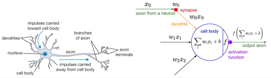
On the left is a picture of neurons, which receive input through synapses and then transmit it to the later neurons through nerve activation. Compared with the neural network on the right, it first receives data input, then obtains the result through calculation, and then passes through the activation function and then transmits it to the neurons in the second layer.

Therefore, the logistic regression model and linear regression model mentioned above can be regarded as a single-layer neural network, and the activation function sigmoid is used in logistic regression.

The activation functions used in neural networks are nonlinear. Each activation function inputs a value, and then makes a specific mathematical operation to get a result. Here are a few examples

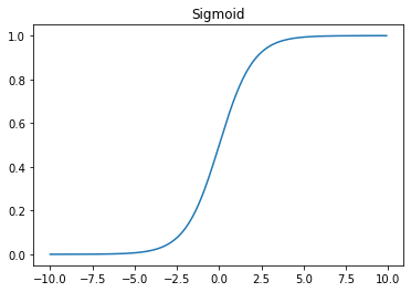
sigmoid activation function

σ ( x ) = 1 1 + e − x \sigma(x) = \frac{1}{1 + e^{-x}} σ(x)=1+e−x1​

def Sigmoid(x):
    return 1 / (1 + np.exp(-x))
    
x = np.arange(-10,10,0.1)    
plt.plot(x, Sigmoid(x),clip_on=False)
plt.title('Sigmoid')

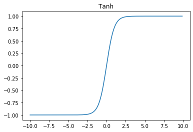
tanh activation function

t a n h ( x ) = 2 σ ( 2 x ) − 1 tanh(x) = 2 \sigma(2x) - 1 tanh(x)=2σ(2x)−1

def Tanh(x):
    return 2 * Sigmoid(2*x) - 1
    
plt.plot(x, Tanh(x))
plt.title('Tanh')

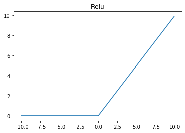
ReLU activation function

R e L U ( x ) = m a x ( 0 , x ) ReLU(x) = max(0, x) ReLU(x)=max(0,x)

def Relu(x):
    return np.maximum(0, x)

plt.plot(x, Relu(x))
plt.title('Relu')

Structure of neural network

Neural network is that many neurons are stacked together to form a layer of neural network. Then multiple layers are stacked together to form a deep neural network. We can show a two-layer neural network and a three-layer neural network through the following figure

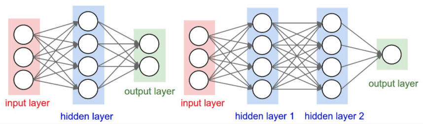
It can be seen that the structure of neural network is very simple, mainly composed of input layer, hidden layer and output layer. The input layer needs to be determined according to the number of features, and the output layer depends on the problem to be solved. Then the number of network layers of hidden layer and the number of neurons in each layer are adjustable parameters, and different layers and parameters of each layer have a great impact on the model

The forward propagation of neural network is also very simple, that is, it is OK to keep doing operations layer by layer. You can take a look at the following example

Why use activation functions

Activation function is very important in neural network, and it is also very necessary to use activation function. Previously, we understood activation function from the perspective of human brain neurons. Because neurons need to be activated to spread back, activation function is needed in neural network. Next, we will understand the necessity of activation function from the perspective of mathematics.

For example, A two-layer neural network uses A to represent the activation function, then

y = w 2 A ( w 1 x ) y = w_2 A(w_1 x) y=w2​A(w1​x)

If we don't use the activation function, the result of the neural network is

y = w 2 ( w 1 x ) = ( w 2 w 1 ) x = w ˉ x y = w_2 (w_1 x) = (w_2 w_1) x = \bar{w} x y=w2​(w1​x)=(w2​w1​)x=wˉx

It can be seen that we combine the parameters of the two-layer neural network w ˉ \bar{w} w ˉ In fact, the two-layer neural network has become one-layer neural network, but the parameters have become new w ˉ \bar{w} w ˉ， So if the activation function is not used, no matter how many layers of neural networks, y = w n ⋯ w 2 w 1 x = w ˉ x y = w_n \cdots w_2 w_1 x = \bar{w} x y=wn​⋯w2​w1​x=w ˉ x. It becomes a single-layer neural network, so we must use the activation function at each layer.

Finally, let's look at the influence of activation function on neural network

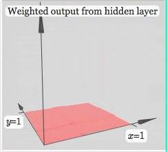
It can be seen that after using the activation function, the neural network can realize any shape by changing the weight. The more complex the neural network can fit, the more complex the shape is. This is the famous universal approximation theorem of neural network.

Let's feel the power of neural network through examples

Second classification problem

import torch
import numpy as np
from torch import nn
from torch.autograd import Variable
import torch.nn.functional as F

import matplotlib.pyplot as plt
%matplotlib inline

Decision boundary

First of all, we define a function of decision boundary, which is convenient for us to draw our decision boundary later. Here we use PLT Contour to draw, because sometimes our function is not a linear function, which is difficult to represent.

def plot_decision_boundary(model, x, y):
    # Set min and max values and give it some padding
    x_min, x_max = x[:, 0].min() - 1, x[:, 0].max() + 1
    y_min, y_max = x[:, 1].min() - 1, x[:, 1].max() + 1
    h = 0.01
    # Generate a grid of points with distance h between them
    xx, yy = np.meshgrid(np.arange(x_min, x_max, h), np.arange(y_min, y_max, h))
    # Predict the function value for the whole grid
    Z = model(np.c_[xx.ravel(), yy.ravel()]) # Get the coordinates of all points
    Z = Z.reshape(xx.shape)
    # Plot the contour and training examples
    plt.contourf(xx, yy, Z, cmap=plt.cm.Spectral) # Sketch contour
    plt.ylabel('x2')
    plt.xlabel('x1')
    plt.scatter(x[:, 0], x[:, 1], c=y.reshape(-1), s=40, cmap=plt.cm.Spectral)

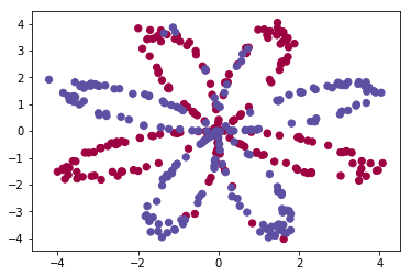
This time we still deal with a binary classification problem, but it is more complex than the previous logistic regression

Randomly generated data

First, we randomly generate some data

np.random.seed(1)
m = 400 # Number of samples
N = int(m/2) # Number of points of each class
D = 2 # dimension
x = np.zeros((m, D))
y = np.zeros((m, 1), dtype='uint8') # label vector, 0 for red, 1 for blue
a = 4

for j in range(2):
    ix = range(N*j,N*(j+1))
    t = np.linspace(j*3.12,(j+1)*3.12,N) + np.random.randn(N)*0.2 # theta
    r = a*np.sin(4*t) + np.random.randn(N)*0.2 # radius
    x[ix] = np.c_[r*np.sin(t), r*np.cos(t)]
    y[ix] = j

plt.scatter(x[:, 0], x[:, 1], c=y.reshape(-1), s=40, cmap=plt.cm.Spectral)

logistic regression solution

x = torch.from_numpy(x).float()
y = torch.from_numpy(y).float()

w = nn.Parameter(torch.randn(2, 1))
b = nn.Parameter(torch.zeros(1))

optimizer = torch.optim.SGD([w, b], 1e-1)

def logistic_regression(x):
    return torch.mm(x, w) + b

criterion = nn.BCEWithLogitsLoss()

for e in range(100):
    out = logistic_regression(Variable(x))
    loss = criterion(out, Variable(y))
    optimizer.zero_grad()
    loss.backward()
    optimizer.step()
    if (e + 1) % 20 == 0:
        print('epoch: {}, loss: {}'.format(e+1, loss.data[0]))

epoch: 20, loss: 0.7033562064170837
epoch: 40, loss: 0.6739853024482727
epoch: 60, loss: 0.6731640696525574
epoch: 80, loss: 0.6731465458869934
epoch: 100, loss: 0.6731461882591248

Result demonstration

def plot_logistic(x):
    x = Variable(torch.from_numpy(x).float())
    out = F.sigmoid(logistic_regression(x))
    out = (out > 0.5) * 1
    return out.data.numpy()

plot_decision_boundary(lambda x: plot_logistic(x), x.numpy(), y.numpy())
plt.title('logistic regression')

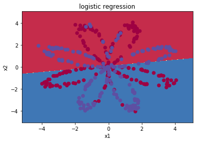
It can be seen that logistic regression can not distinguish this complex data set well. If you remember the previous content, you will know that logistic regression is a linear classifier. It's time for our neural network to appear!

Neural network to solve binary classification problem

# Define the parameters of two-layer neural network
w1 = nn.Parameter(torch.randn(2, 4) * 0.01) # Number of neurons in hidden layer 2
b1 = nn.Parameter(torch.zeros(4))

w2 = nn.Parameter(torch.randn(4, 1) * 0.01)
b2 = nn.Parameter(torch.zeros(1))

# Define model
def two_network(x):
    x1 = torch.mm(x, w1) + b1
    x1 = F.tanh(x1) # Use the tanh activation function of PyTorch
    x2 = torch.mm(x1, w2) + b2
    return x2

optimizer = torch.optim.SGD([w1, w2, b1, b2], 1.)

criterion = nn.BCEWithLogitsLoss()

# We trained 10000 times
for e in range(10000):
    out = two_network(Variable(x))
    loss = criterion(out, Variable(y))
    optimizer.zero_grad()
    loss.backward()
    optimizer.step()
    if (e + 1) % 1000 == 0:
        print('epoch: {}, loss: {}'.format(e+1, loss.data[0]))

def plot_network(x):
    x = Variable(torch.from_numpy(x).float())
    x1 = torch.mm(x, w1) + b1
    x1 = F.tanh(x1)
    x2 = torch.mm(x1, w2) + b2
    out = F.sigmoid(x2)
    out = (out > 0.5) * 1
    return out.data.numpy()

plot_decision_boundary(lambda x: plot_network(x), x.numpy(), y.numpy())
plt.title('2 layer network')

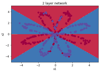
It can be seen that neural network can classify this complex data very well. Compared with the previous logistic regression, neural network has become a nonlinear classifier because of the existence of activation function, so the boundary of neural network classification is more complex.