Introduction to Numpy

NumPy(Numerical Python) is a basic library of scientific computing, which provides a large number of functions related to scientific computing, such as data statistics, random number generation and so on. The core type it provides is multi-dimensional array type (ndarray), which supports a large number of dimensional array and matrix operations. Numpy support vector handles ndarray objects to improve program operation speed.

Numpy (Numerical Python) is an open source Python scientific computing library, which is used to quickly process arrays with arbitrary dimensions.

Numpy supports common array and matrix operations. For the same numerical calculation task, using numpy is much simpler than using Python directly.

Numpy uses the ndarray object to handle multidimensional arrays, which is a fast and flexible big data container.

Introduction to ndarray

NumPy provides an N-dimensional array type, the ndarray,
which describes a collection of "items" of the same type.

NumPy provides an N-dimensional array type ndarray, which describes a collection of "items" of the same type.

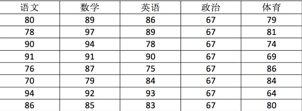
Store with ndarray:

import numpy as np 
# Create ndarray 
score = np.array( 
[[80, 89, 86, 67, 79], 
[78, 97, 89, 67, 81], 
[90, 94, 78, 67, 74], 
[91, 91, 90, 67, 69], 
[76, 87, 75, 67, 86], 
[70, 79, 84, 67, 84], 
[94, 92, 93, 67, 64], 
[86, 85, 83, 67, 80]]) 
score

Return result:

array([[80, 89, 86, 67, 79], 
	  [78, 97, 89, 67, 81], 
	  [90, 94, 78, 67, 74], 
	  [91, 91, 90, 67, 69], 
	  [76, 87, 75, 67, 86], 
	  [70, 79, 84, 67, 84], 
	  [94, 92, 93, 67, 64], 
	  [86, 85, 83, 67, 80]])

put questions to:

Python lists can be used to store one-dimensional arrays, and multi-dimensional arrays can be realized through the nesting of lists. So why use Numpy's ndarray?

Comparison of operation efficiency between ndarray and Python native list

Here we realize the benefits of ndarray by running a piece of code

import random 
import time 
import numpy as np 
a = [] for i in range(100000000): 
a.append(random.random()) 
# Through the% time magic method, view the time taken for the current line of code to run once 
%time sum1=sum(a) 
b=np.array(a) 
%time sum2=np.sum(b)

The first time shows the time calculated using native Python, and the second content is the time calculated using numpy:

CPU times: user 852 ms, sys: 262 ms, total: 1.11 s 
Wall time: 1.13 s

CPU times: user 133 ms, sys: 653 µs, total: 133 ms 
Wall time: 134 ms

From this, we can see that the calculation speed of ndarray is much faster and saves time.

The biggest feature of machine learning is a large number of data operations. Without a fast solution, python may not achieve good results in the field of machine learning.

Numpy is specially designed for ndarray operations and operations, so the storage efficiency and input-output performance of arrays are much better than those of nested lists in Python. The larger the array, the more obvious the advantages of numpy.

Why can darray be so fast?

Advantages of ndarray

Memory block style

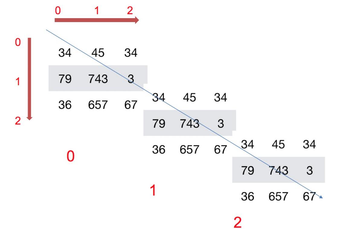
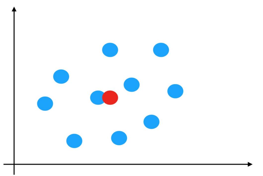
How is ndarray different from the native python list? Please see a figure:

We can see from the figure that when ndarray stores data, the data and data addresses are continuous, which makes the batch operation of array elements faster.

This is because the types of all elements in the ndarray are the same, and the element types in the python list are arbitrary. Therefore, the memory of the ndarray can be continuous when storing elements, while the python native list can only find the next element through addressing. Although this also leads to the fact that the ndarray of numpy is inferior to the python native list in terms of general performance, in scientific calculation, Numpy's ndarray can eliminate many circular statements, and the code is much simpler than Python's native list.

ndarray supports parallelization (vectorization)

Numpy has built-in parallel computing function. When the system has multiple cores, numpy will automatically perform parallel computing when doing some computing

Much more efficient than pure Python code

The bottom layer of Numpy is written in C language, and the GIL (global interpreter lock) is released internally. Its operation speed on the array is not limited by the Python interpreter. Therefore, its efficiency is much higher than that of pure Python code.

Numpy installation

The easiest way to install NumPy is to use the pip tool. The syntax format is as follows:

pip install numpy

arange function test environment installation

import numpy as np 
a=np.arange(10) 
print(a)

In the above program, only an orange function in the numpy module is involved. This function can pass in an integer type parameter n. The return value of the function looks like a list. In fact, the return value type is numpy ndarray. This is a unique array type in numpy. If the parameter value passed into the range function is n, the range function returns an array of ndarray types from 0 to n-1.

N-dimensional array - ndarray

array creation

The array function of numpy module can generate multi-dimensional arrays. For example, if you want to generate a two-dimensional array, you need to pass a list type parameter to the array function. Each list element is a one-dimensional array of ndarray type as the row of the two-dimensional array. In addition, the number of elements in each dimension of the array (in tuple form) can be obtained through the shape attribute of the ndarray class, or the number of elements in each dimension can be obtained in the form of shape[n], where n is the dimension, starting from 0.

The syntax format is as follows:

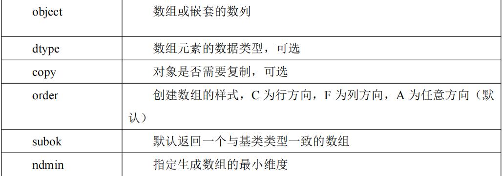
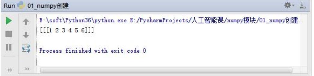
Use of ndmin parameter

import numpy as np 
a=np.array([1,2,3,4,5,6],ndmin=3) 
print(a)

Use of dtype parameters

a=np.array([1,2,3,4,5,6],dtype=complex) 
print(a)

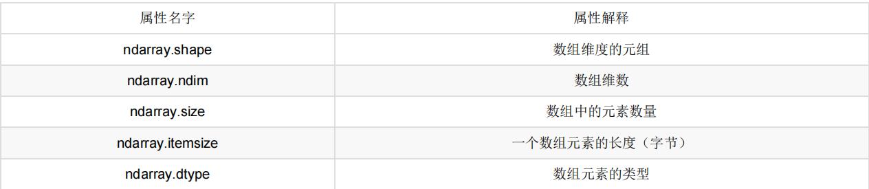
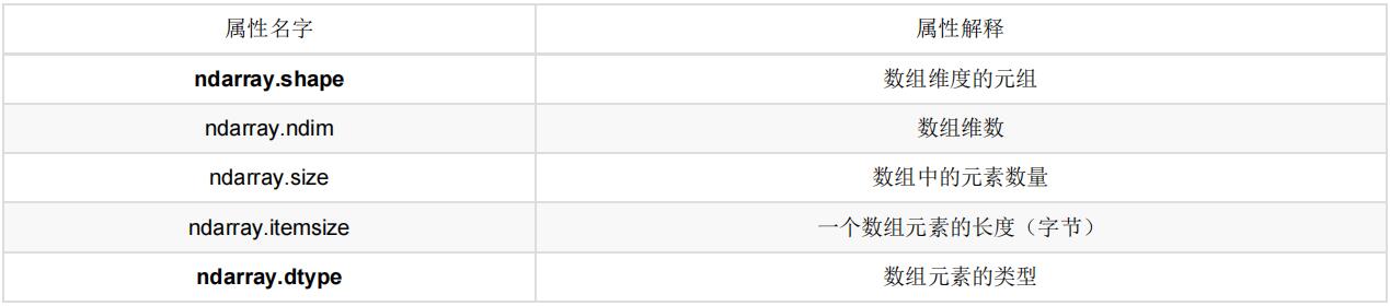
Properties of ndarray

Array properties reflect the information inherent in the array itself.

Shape of ndarray

First create some arrays.

# Create arrays of different shapes 
>>> a = np.array([[1,2,3],[4,5,6]]) 
>>> b = np.array([1,2,3,4]) 
>>> c = np.array([[[1,2,3],[4,5,6]],[[1,2,3],[4,5,6]]])

Print out shapes separately

>>> a.shape 
>>> b.shape 
>>> c.shape 
(2, 3) # Two dimensional array 
(4,) # One dimensional array 
(2, 2, 3) # 3D array

How to understand the shape of an array?

2D array:

3D array:

Type of ndarray

>>> type(score.dtype) 
<type 'numpy.dtype'>

dtype is numpy dtype type, first look at the types of arrays:

Specify the type when creating an array

>>> a = np.array([[1, 2, 3],[4, 5, 6]], dtype=np.float32) >>> a.dtype 
dtype('float32') 

>>> arr = np.array(['python', 'tensorflow', 'scikit-learn', 'numpy'], dtype = np.string_) 
>>> arr 
array([b'python', b'tensorflow', b'scikit-learn', b'numpy'], dtype='|S12')

Note: if not specified, integer defaults to int64 and decimal defaults to float64

summary

Basic properties of array

basic operation

Method of generating array

Generate an array of 0 and 1

np.ones(shape, dtype)
np.ones_like(a, dtype)
np.zeros(shape, dtype)
np.zeros_like(a, dtype)

ones = np.ones([4, 8])
ones

array([[1., 1., 1., 1., 1., 1., 1., 1.],
       [1., 1., 1., 1., 1., 1., 1., 1.],
       [1., 1., 1., 1., 1., 1., 1., 1.],
       [1., 1., 1., 1., 1., 1., 1., 1.]])

np.zeros_like(ones)

array([[0., 0., 0., 0., 0., 0., 0., 0.],
       [0., 0., 0., 0., 0., 0., 0., 0.],
       [0., 0., 0., 0., 0., 0., 0., 0.],
       [0., 0., 0., 0., 0., 0., 0., 0.]])

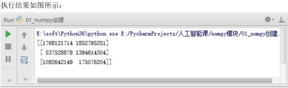
np.empy()

numpy. The empty method is used to create an uninitialized array with a specified shape and data type. The value of the element in the array is the value of the previous memory:

numpy.empty(shape, dtype = float, order = 'C')

empty create

x=np.empty([3,2],dtype=int) 
print(x)

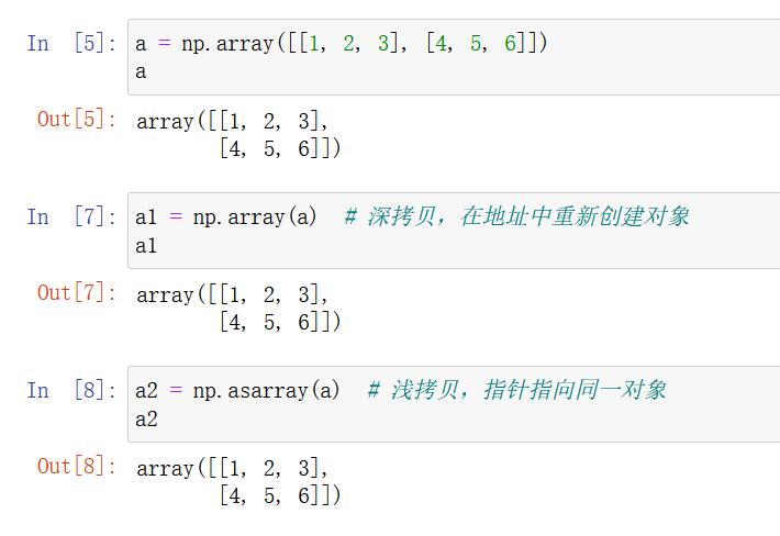
Generate from existing array

Generation mode

np.array(object, dtype)
np.asarray(a, dtype)

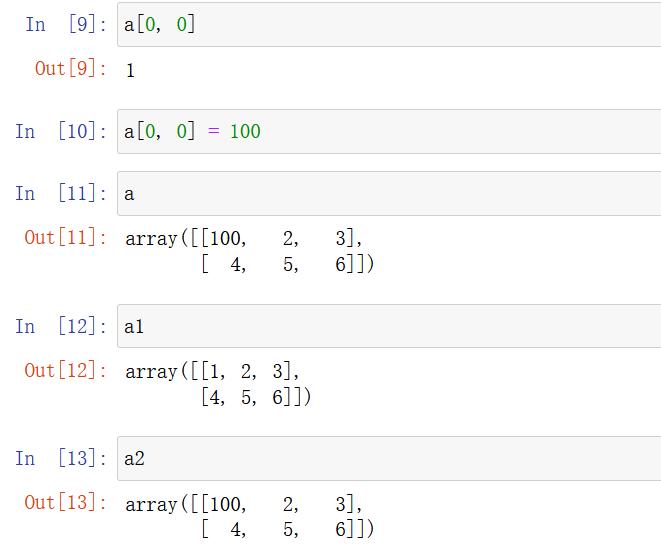
a = np.array([[1,2,3],[4,5,6]]) 
# Create from an existing array 
a1 = np.array(a) 
# Equivalent to the form of an index, there is no real creation of a new one 
a2 = np.asarray(a)

About the difference between array and asarray

Generate a fixed range array

np.linspace (start, stop, num, endpoint)

np.linspace(start, stop, num=50, endpoint=True, retstep=False, dtype=None)

• Create an isometric array - specify the number
• Parameters:
  • start: the starting value of the sequence
  • stop: the end value of the sequence
  • num: the number of equally spaced samples to be generated. The default value is 50
  • endpoint: whether the sequence contains the stop value. The default value is true
  • retstep: if True, the spacing will be displayed in the generated array, otherwise it will not be displayed.
  • Dtype: data type of ndarray

# Generate equally spaced arrays 
np.linspace(0, 100, 11)

Return result:

array([ 0., 10., 20., 30., 40., 50., 60., 70., 80., 90., 100.])

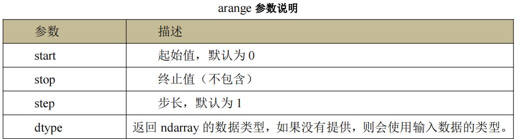
np.arange(start,stop, step, dtype)

• Create an isometric array - specify the step size
• parameter
  • Step: step size. The default value is 1

np.arange(10, 50, 2)

Return result:

array([10, 12, 14, 16, 18, 20, 22, 24, 26, 28, 30, 32, 34, 36, 38, 40, 42, 44, 46, 48])

np.logspace(start,stop, num)

• Create an isometric sequence
• Parameters:
  • num: the number of proportional series to be generated. The default value is 50

# Generate 10^x 
np.logspace(0, 2, 3)

Return result:

array([ 1., 10., 100.])

Generate random array

Introduction to using module: NP Random module

Normal distribution

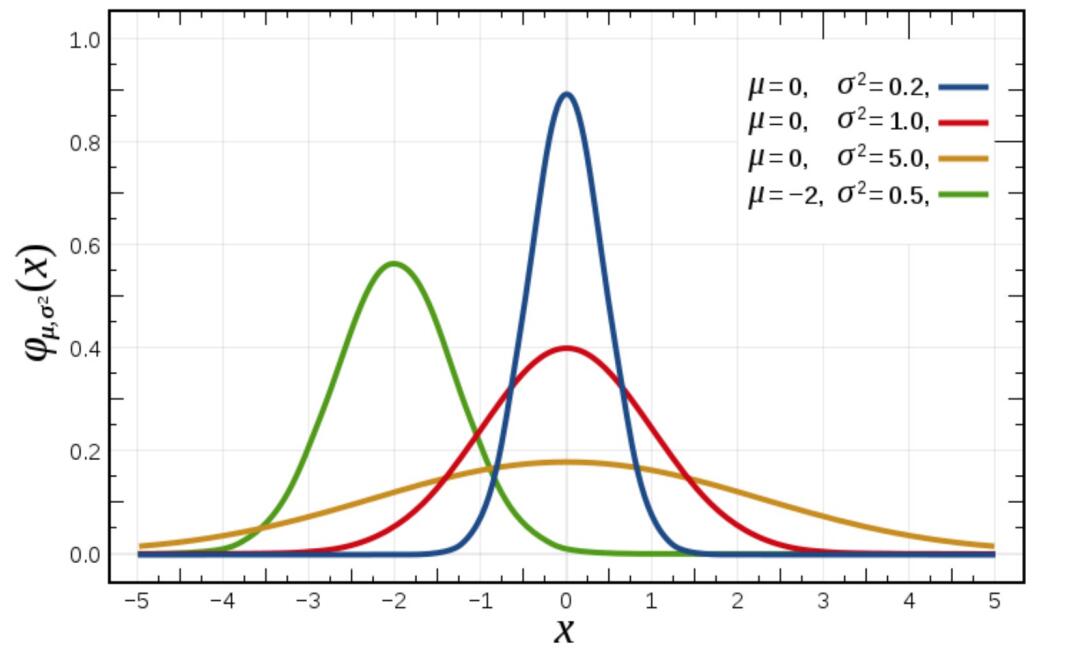
What is normal distribution?

Normal distribution is a probability distribution. The normal distribution has two parameters μ and σ Distribution of continuous random variables, first parameter μ Is the mean value of random variables subject to normal distribution, the second parameter σ Is the standard deviation of this random variable, so the normal distribution is recorded as n( μ，σ ).

Application of normal distribution

The probability distribution of many random variables in life, production and scientific experiments can be approximately described by normal distribution.

Normal distribution characteristics

μ Determines its position and its standard deviation σ Determines the magnitude of the distribution. When μ = 0 σ = The normal distribution at 1 is the standard normal distribution.

How does the standard deviation come from?

• variance
  It is a measure of the degree of dispersion when probability theory and statistical variance measure a set of data
  
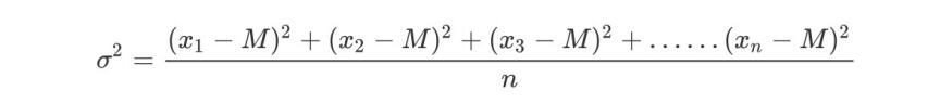
  Where M is the average value and n is the total number of data, σ Is the standard deviation, σ ^ 2 it can be understood that a whole is variance

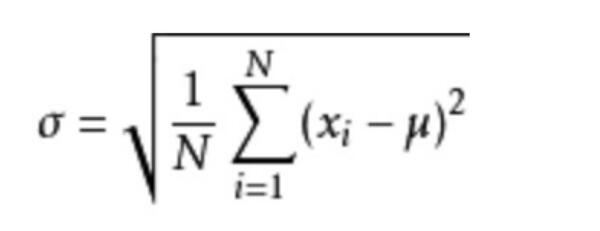
• Significance of standard deviation and variance
  It can be understood as a measure of the degree of dispersion of data

Normal distribution creation method

• np.random.randn(d0, d1, ..., dn)
  Function: return one or more sample values from standard normal distribution
• np.random.normal(loc=0.0, scale=1.0, size=None)

loc: float
The mean value of this probability distribution (corresponding to the center of the whole distribution)
scale: float
The standard deviation of this probability distribution (corresponding to the width of the distribution, the larger the scale, the fatter, and the smaller the scale, the thinner)
size: int or tuple of ints
The output shape is None by default, and only one value is output
np.random.standard_normal(size=None)
Returns an array of standard normal distributions for a specified shape.

Example 1: generate 100000000 normal distribution data with mean value of 1.75 and standard deviation of 1

x1 = np.random.normal(1.75, 1, 100000000)

Return result:

array([2.90646763, 1.46737886, 2.21799024, ..., 1.56047411, 1.87969135, 0.9028096 ])

# 1. Create canvas
plt.figure(figsize=(20, 8), dpi=100)

# 2. Draw image
plt.hist(x1, 1000)  # 1000 groups

# 3. Display image
plt.show()

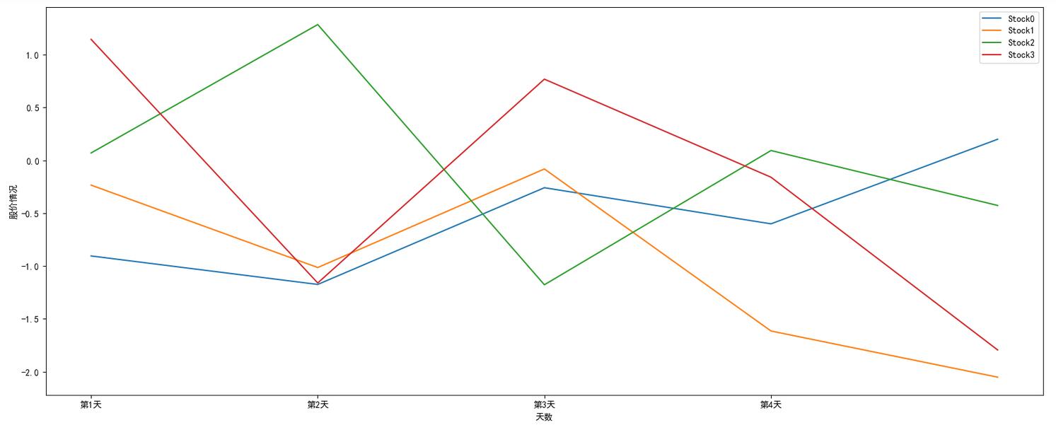
For example, we can simulate the data of the rise and fall of a group of stocks

Example 2: randomly generate the daily increase data of four stocks for one week

How to obtain the weekly (5-day) fluctuation data of 4 stocks?

• Randomly generated rise and fall within a normal distribution, such as mean 0 and variance 1

Creation of stock fluctuation data

# Create 5-day rise and fall data of 4 stocks in line with normal distribution
stock_change = np.random.normal(0, 1, (4, 5)) 
stock_change

array([[-0.90442265, -1.17400313, -0.25891122, -0.60057691,  0.19973249],
       [-0.23449971, -1.01396609, -0.08161324, -1.61459823, -2.05132145],
       [ 0.0700032 ,  1.28480273, -1.17703456,  0.0929877 , -0.42675005],
       [ 1.14477016, -1.16018108,  0.76815853, -0.15971892, -1.79386421]])

# 1. Create canvas
plt.figure(figsize=(20, 8), dpi=100)

days = ['one', 'two', ]
# 2. Draw images and multi maps
for i in range(len(stock_change)):
    plt.plot(stock_change[i], label='Stock'+str(i))

# 2.1. Set x-axis scale
days = ['The first{}day'.format(i+1) for i in range(0, 4)]
plt.xticks(range(0, 4), days)

# 2.2. Set x, y axis labels
plt.xlabel('Days')
plt.ylabel('Share price')

# 2.3 setting legend
plt.legend(loc=0)

# 3. Display image
plt.show()

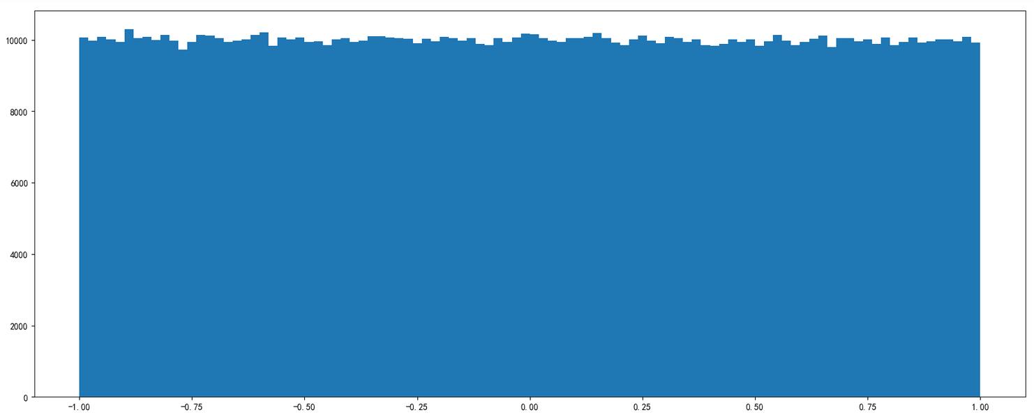
uniform distribution

• np.random.rand(d0, d1, ..., dn)
  • Returns a set of evenly distributed numbers in [0.0, 1.0).
• np.random.uniform(low=0.0, high=1.0, size=None)
  • Function: randomly sample from a uniform distribution [low, high]. Note that the definition domain is closed left and open right, that is, it contains low and does not contain high
  • Parameter introduction:
    • low: sampling lower bound, float type, the default value is 0;
    • high: sampling upper bound, float type, the default value is 1;
    • Size: the number of output samples, which is of type int or tuple. For example, if size=(m,n,k), mnk samples will be output, and 1 value will be output by default.
  • Return value: ndarray type, whose shape is consistent with that described in the parameter size.
• np.random.randint(low, high=None, size=None, dtype='l')
  • Randomly sample from a uniform distribution to generate an integer or N-dimensional integer array,
  • Access range: if high is not None, the random integer between [low, high]) is taken; otherwise, the random integer between [0, low]) is taken.

# Generate uniformly distributed random numbers 
x2 = np.random.uniform(-1, 1, 100000000)

Return result:

array([ 0.22411206, 0.31414671, 0.85655613, ..., -0.92972446, 0.95985223, 0.23197723])

Draw a picture to see the distribution:

# 1. Create canvas
plt.figure(figsize=(20, 8), dpi=100)

# 2. Draw image
plt.hist(x2, 1000)  # 1000 groups

# 3. Display image
plt.show()

Index and slice of array

The contents of the ndarray object can be accessed and modified by indexing or slicing, just like the slicing operation of list in Python.

The ndarray array can be indexed based on the subscript of 0 - n, and set the start, stop and step parameters to cut a new array from the original array.

How to index one-dimensional, two-dimensional and three-dimensional arrays?

• Direct indexing, slicing
• Object [:,:] – first and last columns

Two dimensional array index method:

• For example: obtain the rise and fall data of the first stock in the first three trading days

# Two dimensional array, two dimensions 
stock_change[0, 0:3]

Return result:

array([-0.03862668, -1.46128096, -0.75596237])

3D array index method:

# three-dimensional 
a1 = np.array([ [[1,2,3],[4,5,6]], [[12,3,34],[5,6,7]]]) 
# Return results 
array([[[ 1, 2, 3], [ 4, 5, 6]],
	  [[12, 3, 34], [ 5, 6, 7]]])
# Index, slice 
>>> a1[0, 0, 1] # Output: 2

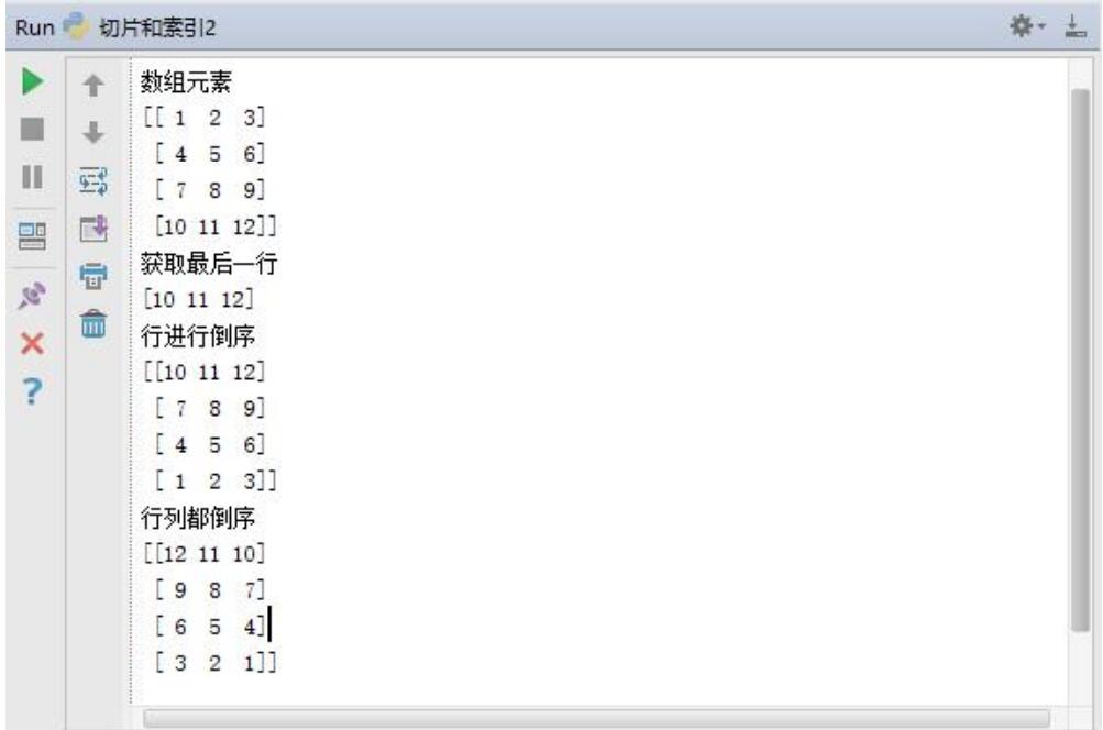
Index is negative to get

print('Get last row') 
print(a[-1]) 
print('Reverse the order of rows')
print(a[::-1]) 
print('The ranks are in reverse order') 
print(a[::-1,::-1])

Shape modification

An important task in processing arrays is to change the dimensions of the array, including increasing and decreasing the dimensions of the array, as well as the transpose of the array. Numpy provides a large number of API s that can easily complete the operation of these arrays. For example, a one-dimensional array can be changed into a two-dimensional, three-dimensional or multi-dimensional array through the reshape method. The multi-dimensional array can be changed into one-dimensional array through the t ravel method or the flatten method. To change the dimension of the array, you can also directly set the shape attribute (tuple type) of the numpy array. You can also change the dimension of the array through the resize method.

ndarray.reshape(shape, order)

• Returns a view with the same data field but different shape s
• Rows and columns are not interchangeable

# When converting shapes, be sure to pay attention to the element matching of the array 
stock_change.reshape([5, 4]) 
stock_change.reshape([-1,10]) # The shape of the array is modified to: (2, 10), - 1: indicates that it passes through the to be calculated

ndarray.resize(new_shape)

• Modify the shape of the array itself (keep the number of elements the same)
• Rows and columns are not interchangeable

stock_change.resize([5, 4]) 

# View modified results 
stock_change.shape 
(5, 4)

ndarray.T

• Transpose of array
• Exchange the rows and columns of the array

stock_change.T.shape 
(4, 5)

ndarray.ravel

#Use the t ravel function to turn a three-dimensional b into a one-dimensional array
a1=b.ravel()
print(a1)
print('-'*30)

ndarray.flatten

#Use the flatten function to turn a two-dimensional c into a one-dimensional array 
a2=c.flatten() 
print(a2) 
print('-'*30)

Type modification

ndarray.astype(type)

• Returns the array after the type is modified\

stock_change.astype(np.int32)

ndarray.tostring([order]) or ndarray tobytes([order])

Construct Python bytes that contain the original data bytes in the array

arr = np.array([[[1, 2, 3], [4, 5, 6]], [[12, 3, 34], [5, 6, 7]]]) 
arr.tostring()

Too large jupyter output may cause crash problems

If encountered

IOPub data rate exceeded. The notebook server will temporarily stop sending output to the client in order to avoid crashing it. To change this limit, set the config variable --NotebookApp.iopub_data_rate_limit.

The problem is that there is a limit on the number of bytes output in jupyer. You need to modify the configuration file:

create profile

jupyter notebook --generate-config 
vi ~/.jupyter/jupyter_notebook_config.py

Uncomment and add more

## (bytes/sec) Maximum rate at which messages can be sent on iopub before they 
# are limited. 
c.NotebookApp.iopub_data_rate_limit = 10000000

However, it is not recommended to modify it in this way. The output of jupyter will crash if it is too large

Array de duplication

np.unique()

temp = np.array([[1, 2, 3, 4],[3, 4, 5, 6]]) 
>>> np.unique(temp) 
array([1, 2, 3, 4, 5, 6])

Darray operation

Logical operation

# Generate data for 10 students and 5 courses 
>>> score = np.random.randint(40, 100, (10, 5)) 

# Take out the scores of the last four students for logical judgment 
>>> test_score = score[6:, 0:5] 

# Logical judgment. If the score is greater than 60, it is marked as True; otherwise, it is False 
>>> test_score > 60 
array([[ True, True, True, False, True], [ True, True, True, False, True], [ True, True, False, False, True], [False, True, True, True, True]]) 

# BOOL assignment, which sets the satisfying condition to the specified value - Boolean index 
>>> test_score[test_score > 60] = 1 
>>> test_score 
array([[ 1, 1, 1, 52, 1], 
	  [ 1, 1, 1, 59, 1], 
	  [ 1, 1, 44, 44, 1], 
	  [59, 1, 1, 1, 1]])

General judgment function

np.all()

# Judge whether the first two students have passed [0:2,:] 
>>> np.all(score[0:2, :] > 60) 
False

np.any()

# Judge whether the score of the first two students [0:2,:] is greater than 90 
>>> np.any(score[0:2, :] > 80) 
True

np.where (ternary operator)

By using NP Where can perform more complex operations

# Judge the top four students. In the top four courses, the score greater than 60 is set as 1, otherwise it is 0 
temp = score[:4, :4] 
np.where(temp > 60, 1, 0)

Compound logic needs to be combined with NP logical_ And and NP logical_ Or use

# Judge the top four students. In the first four courses, the score greater than 60 and less than 90 is changed to 1, otherwise it is 0 
np.where(np.logical_and(temp > 60, temp < 90), 1, 0) 

# Judge the top four students. In the first four courses, the score greater than 90 or less than 60 is changed to 1, otherwise it is 0 
np.where(np.logical_or(temp > 90, temp < 60), 1, 0)

Statistical operation

What should I do if I want to know the student's maximum score or make a small score?

statistical indicators

In the field of data mining / machine learning, the value of statistical indicators is also a way for us to analyze problems. Common indicators are as follows:

Case: student achievement statistical operation

During statistics, the value of axis is not necessarily the same. The values of different API axes in Numpy are different. Here, axis 0 represents a column and axis 1 represents a row for statistics

# Next, for the top four students, do some statistical operations 
# Specify column de statistics 
temp = score[:4, 0:5] 
print("Top four students,Maximum score of each subject:{}".format(np.max(temp, axis=0))) 
print("Top four students,Minimum score of each subject:{}".format(np.min(temp, axis=0))) 
print("Top four students,Performance fluctuation of each subject:{}".format(np.std(temp, axis=0))) 
print("Top four students,Average score of each subject:{}".format(np.mean(temp, axis=0)))

result:

Top four students,Maximum score of each subject:[96 97 72 98 89] 
Top four students,Minimum score of each subject:[55 57 45 76 77] 
Top four students,Performance fluctuation of each subject:[16.25576821 14.92271758 10.40432602 8.0311892 4.32290412] 
Top four students,Average score of each subject:[78.5 75.75 62.5 85. 82.25]

If it is necessary to calculate which student has the highest score in a subject?

• np.argmax(temp, axis=)
• np.argmin(temp, axis=)

print("For the top four students, the subscript of the student with the highest score in each subject:{}".format(np.argmax(temp, axis=0)))

result:

For the top four students, the subscript of the student with the highest score in each subject:[0 2 0 0 1]

Array separator

split separation

numpy. The split function divides an array into subarrays along a specific axis. The format is as follows:

numpy.split(ary, indices_or_sections, axis)

Parameter Description:

ary: array to be split
indices_or_sections: if it is an integer, the number is used to divide evenly. If it is an array, it is the position along the axis.
axis: along which dimension is the tangent, the default value is 0, and the horizontal tangent is 0. When it is 1, vertical segmentation.

split separated one-dimensional array

import numpy as np 
x=np.arange(1,9) 
a=np.split(x,4) 
print(a) 
print(a[0]) 
print(a[1]) 
print(a[2]) 
print(a[3]) 

#Passing arrays for separation 
b=np.split(x,[3,5]) 
print(b)

split separated two-dimensional array

#Import numpy
import numpy as np 
#Create two arrays 
a=np.array([[1,2,3],[4,5,6],[11,12,13],[14,15,16]]) 
print('axis=0 Vertical average separation') 
r=np.split(a,2,axis=0) 
print(r[0]) 
print(r[1]) 
print('axis=1 The horizontal direction is separated by position') 
r=np.split(a,[2],axis=1) 
print(r)

Horizontally separated array

Separated array is the inverse process of combined array. Like combined array, separated array is also divided into horizontal separated array and vertical separated array. The horizontally separated array corresponds to the horizontally combined array. Horizontal combined array is to end and connect two or more arrays horizontally, while horizontal separated array is to separate the arrays that have been combined horizontally.

The hsplit function can be used to horizontally separate arrays. The function has two parameters. The first parameter represents the array to be separated, and the second parameter represents that the array should be horizontally separated into several small arrays. Now let's take a look at an example.

The following is a 2 * 6 two-dimensional array X

Now, array X is separated into three arrays with 2 columns. However, if hsplit(X,4) is used to separate array X, an exception will be thrown. This is because array X cannot be separated into four arrays with the same number of columns. Therefore, a rule for separating arrays using hsplit function is that the second parameter value must be able to divide the number of columns of the array to be separated.

hsplit

grid=np.arange(16).reshape(4,4) 
a,b=np.hsplit(grid,2) 
print(a) 
print(b)

Vertically separated array

Vertically separating arrays is the inverse process of vertically combining arrays. Vertically combined arrays connect two or more arrays vertically, and vertically separated arrays separate the arrays that have been vertically combined.

vsplit function can be used to vertically separate arrays. The function has two parameters. The first parameter represents the array to be separated, and the second parameter represents the vertical separation of the array into several small arrays.

As an example, a 4 * 3 two-dimensional array X.

vsplit

grid=np.arange(16).reshape(4,4) 
a,b=np.vsplit(grid,[3]) 
print(a) 
print(b) 
print('tripartite'*10) 
a,b,c=np.vsplit(grid,[1,3]) 
print(a) 
print(b) 
print(c)

transpose

#transpose
#2D transpose 
a=np.arange(1,13).reshape(2,6) 
print('Original array a') 
print(a) 
print('Transposed array') 
print(a.transpose()) 
#Multidimensional array transpose 
aaa=np.arange(1,37).reshape(1,3,3,4) 
#Convert 1,3,3,4 to 3,3,4,1 
print(np.transpose(aaa,[1,2,3,0]).shape)

Inter array operation

Arithmetic function

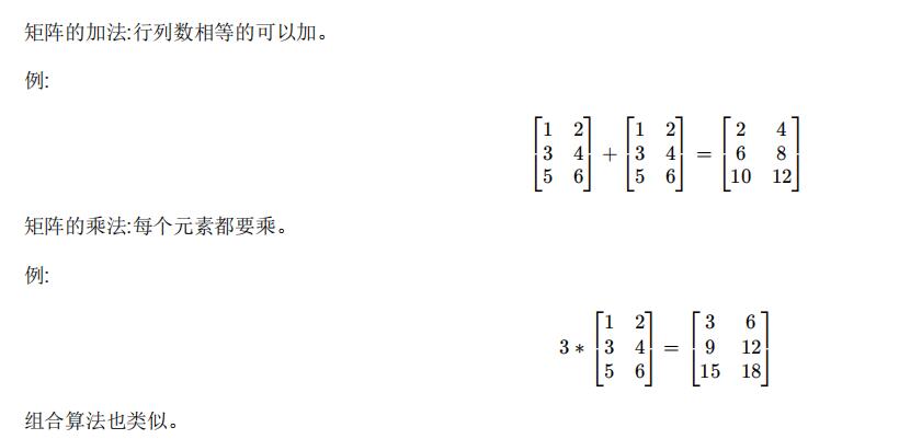
If both objects involved in the operation are ndarray and have the same shape, the bits will be (+ - * /) operated on each other. NumPy arithmetic functions contain simple addition, subtraction, multiplication and division: add(), subtract(), multiply(), and divide().

Mathematical function

NumPy provides standard trigonometric functions: sin(), cos(), tan().

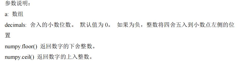
numpy. The around() function returns the rounded value of the specified number.

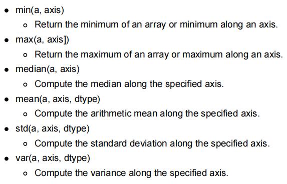
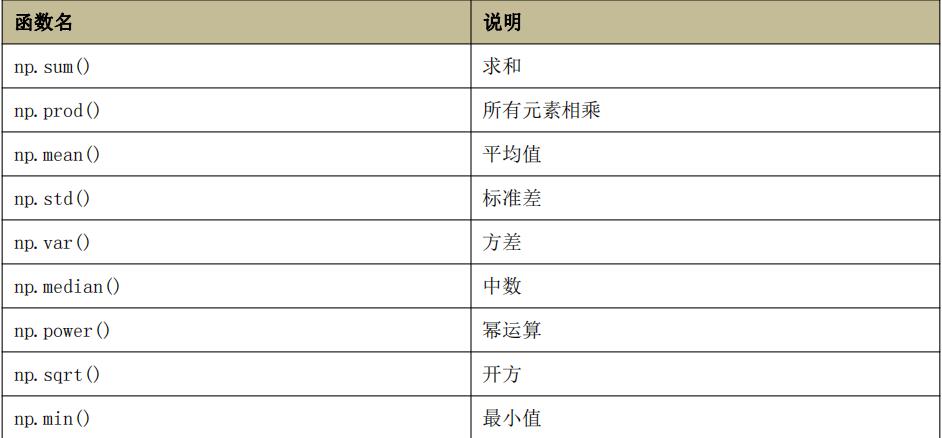
Aggregate function

NumPy provides many statistical functions to find the minimum element, maximum element, percentile standard deviation and variance from the array. The details are as follows:

numpy. The mean() function returns the arithmetic mean of the elements in the array. If an axis is provided, the arithmetic mean calculated along it is the sum of the elements along the axis divided by the number of elements.

numpy. The power() function takes the element in the first input array as the base and calculates its power to the corresponding element in the second input array.

Reference code:

# Import numpy module
import numpy as np

a = np.arange(9).reshape(3, 3)
b = np.array([10, 10, 10])
print('addition')
print(np.add(a, b))
print((a+b))

print('subtraction')
print(np.subtract(b, a))
print(b-a)

# Use of out parameter
y = np.empty((3, 3), dtype=np.int)
np.multiply(a, 10, out=y)
print(y)

# Mathematical function
a = np.array([0, 30, 60, 90])
print(np.sin(a))

# around ceil floor
a = np.array([1.0, 4.55, 123, 0.567, 25.532])
print('around:', np.round(a))
print('ceil:', np.ceil(a))
print('floor', np.floor(a))

# Statistical function
# power
a = np.arange(1, 13).reshape(3, 4)
print('Primitive function a')
print(a)
print('power', np.power(a, 2))

# Use of out in power
x = np.arange(5)
y = np.zeros(10)
np.power(2, x, out=y[:5])
print(y)

# median()
# Median of one-dimensional array
a = np.array([4, 3, 2, 5, 2, 1])  # Sort the array [1,2,2,3,4,5] the number of elements in the array is even, and the median refers to the average of the middle two numbers
print(np.median(a))

a=np.array([4, 3, 2, 5, 2])  # Sort the array [2,2,3,4,5] the number of elements in the array is odd, and the median refers to the number in the middle
print(np.median(a))

# The axis of a two-dimensional array should be specified through axis
a = np.arange(1, 13).reshape(3, 4)
print(a)
print('vertical direction', np.median(a, axis=0))
print('horizontal direction', np.median(a, axis=1))

# mean average
# One dimensional array
a = np.array([4, 3, 2, 5, 2])
print(np.mean(a))

# The two-dimensional array axis specifies the average of the axes
a = np.arange(13).reshape(3, 4)
print(a)
print('axis=0 vertical direction', np.mean(a, axis=0))
print('axis=1 horizontal direction', np.mean(a, axis=1))

# sum() max() min()
a = np.array([4, 3, 2, 5, 2])
print('max:', np.max(a))
print('sum:', np.sum(a))
print('min:', np.min(a))

# argmax argmin: gets the index of the highest value
print('argmin:', np.argmin(a))
print('argmax:', np.argmax(a))

Operation of array and number

arr = np.array([[1, 2, 3, 2, 1, 4], [5, 6, 1, 2, 3, 1]]) 
arr + 1 
arr / 2 

# You can compare the operations of python list to see the difference 
a = [1, 2, 3, 4, 5] 
a * 3

Array and array operation

arr1 = np.array([[1, 2, 3, 2, 1, 4], [5, 6, 1, 2, 3, 1]]) 
arr2 = np.array([[1, 2, 3, 4], [3, 4, 5, 6]])

Broadcasting mechanism

When the array is vectorized, the shape of the array is required to be equal. When arrays with unequal shapes perform arithmetic operations, a broadcast mechanism will appear. This mechanism will expand the array to make the shape attribute value of the array the same. In this way, vectorization operation can be carried out. The following is an example:

arr1 = np.array([[0],[1],[2],[3]]) 
arr1.shape 
# (4, 1) 

arr2 = np.array([1,2,3]) 
arr2.shape 
# (3,) 
arr1+arr2 
# The result is: 
array([[1, 2, 3], 
	   [2, 3, 4], 
	   [3, 4, 5], 
	   [4, 5, 6]])

In the above code, array arr1 is 4 rows and 1 column, and arr2 is 1 row and 3 columns. The two arrays should be added. According to the broadcast mechanism, both arrays arr1 and arr2 will be extended, so that both arrays arr1 and arr2 become 4 rows and 3 columns.

This sentence is the core of understanding broadcasting. Broadcasting mainly occurs in two cases: one is that the dimensions of two arrays are not equal, but the axis lengths of their trailing edge dimensions are consistent, and the other is that the length of one side is 1.

The broadcast mechanism realizes the operation of two or more arrays. Even if the shape s of these arrays are not exactly the same, it only needs to meet any of the following conditions.

• If the axis lengths of the trailing dimension (i.e. the dimension from the end) of the two arrays match,
• Or one of them has a length of 1.

The broadcast mechanism will be on the dimension of missing and / or length 1.

The broadcast mechanism needs to expand the array with small dimension to make it the same as the shape value of the array with the largest dimension, so as to use element level functions or operators for operation.

If this is the case, there is no match:

A (1d array): 10 
B (1d array): 12 
A (2d array): 2 x 1 
B (3d array): 8 x 4 x 3

These two can

arr1 = np.array([[1, 2, 3, 2, 1, 4], [5, 6, 1, 2, 3, 1]]) 
arr2 = np.array([[1], [3]])

Array splicing

Horizontal array combination

Through the hstack function, two or more arrays can be combined horizontally to form an array. What is the horizontal combination of arrays.

Now there are two 2 * 3 arrays A and B.

As you can see, array A and array B are connected horizontally to form a new array. This is the horizontal combination of arrays. The effect of horizontal combination of multiple arrays is similar. However, the horizontal combination of arrays must meet one condition, that is, the number of rows of all arrays participating in the horizontal combination must be the same, otherwise the horizontal combination will throw an exception.

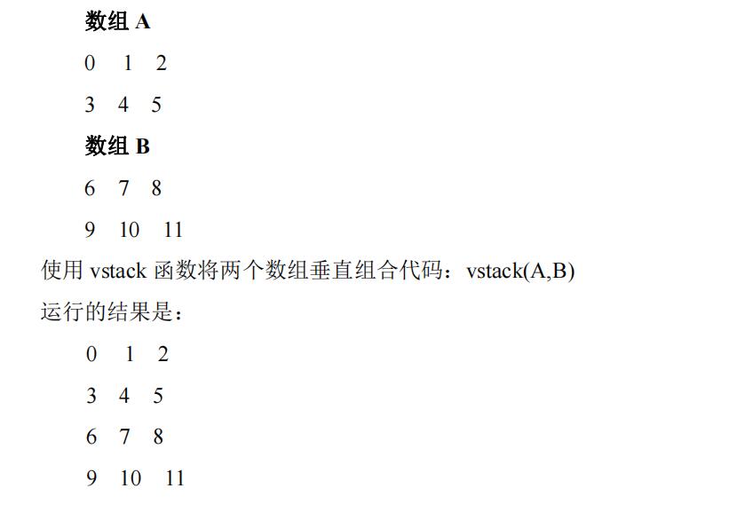
Vertical array combination

Through vstack function, two or more arrays can be vertically combined to form an array. What is the vertical combination of arrays?

Now take two 2 * 3 arrays A and B as an example

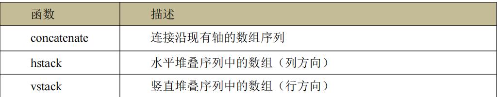
concatenate

numpy. The concatenate function is used to connect two or more arrays of the same shape along the specified axis. The format is as follows:

numpy.concatenate((a1, a2, ...), axis)

Parameter Description:
a1, a2, ...: Arrays of the same type
Axis: the axis along which the array is connected. The default value is 0

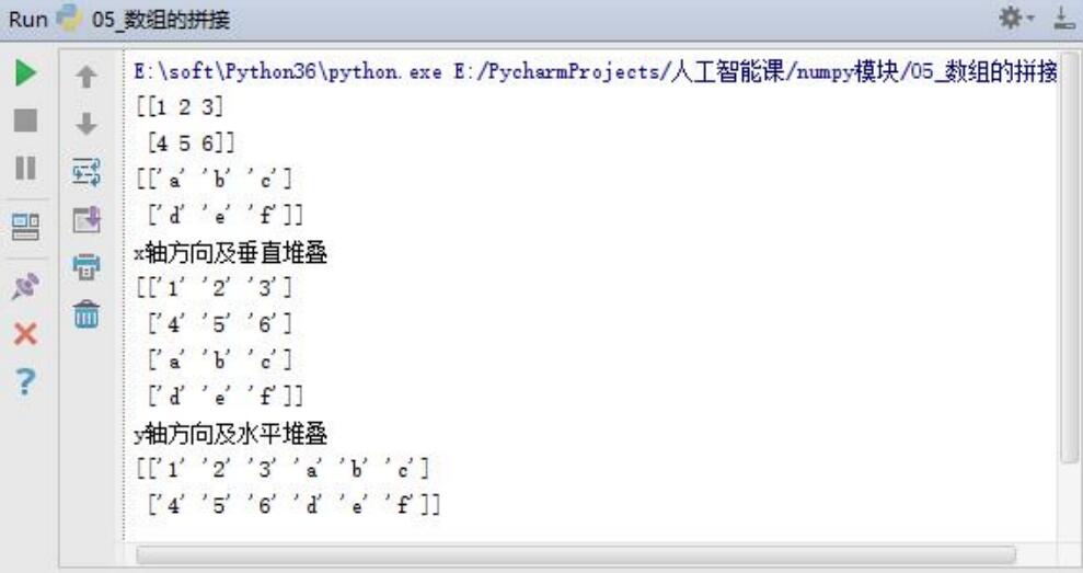
concatenate to realize the splicing of arrays

a=np.array([[1,2,3],[4,5,6]]) 
print(a) 
b=np.array([['a','b','c'],['d','e','f']]) 
print(b) 
print(np.concatenate([a,b]))

print('Vertical splicing is equivalent to vstack') 
print(np.concatenate([a,b],axis=0)) 
print('Horizontal splicing is equivalent to hstack') 
print(np.concatenate([a,b],axis=1))

hstack&vstack

numpy. Hsstack, which generates arrays by stacking horizontally.
numpy.vstack generates arrays by stacking vertically.

vstack and hstack realize array splicing

print('x Axial direction and vertical stacking') 
print(np.vstack([a,b])) 
print('y Axial direction and horizontal stacking') 
print(np.hstack([a,b]))

Note that if the number of rows and columns spliced is different, an error will be reported

Splicing of 3D arrays

aa=np.arange(1,37).reshape(3,4,3) 
print(aa) 
bb=np.arange(101,137).reshape(3,4,3) 
print(bb) 
print('axis=0'*10) 
print(np.concatenate((aa,bb),axis=0)) #6 4 3 
print('axis=1'*10) 
print(np.concatenate((aa,bb),axis=1)) #3,8,3 
print('axis=2'*10) 
print(np.concatenate((aa,bb),axis=2)) #3,4,6

axis=0 can be replaced with vstack
axis=1 can be replaced with hstack
axis=2 can be replaced with dstack

Mathematics: matrix

matrix

The difference between matrix, English matrix and array must be two-dimensional, but array can be multi-dimensional.

As shown in the figure: This is 3 × 2 matrix, that is, 3 rows and 2 columns. If m is row and n is column, then m × n is 3 × two

The dimension of a matrix is the number of rows × Number of columns

Matrix element (matrix item):

Aij refers to the element in row i and column j.

vector

Vector is a special matrix. The vectors in the handout are generally column vectors. The following is a three-dimensional column vector (3) × 1).

Addition and Scalar Multiplication

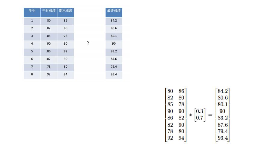
matrix-vector multiplication

The multiplication of matrix and vector is shown in the figure: m × The matrix of N times n × The vector of 1 gets m × Vector of 1

Example:

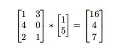
1 * 1+3 * 5 = 16
4 * 1+0 * 5 = 4
2 * 1+1 * 5 = 7

Matrix multiplication follows the following guidelines:

(row M, column N) * (row N, column L) = (row M, column L)

Matrix multiplication

Properties of matrix multiplication

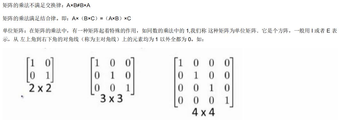
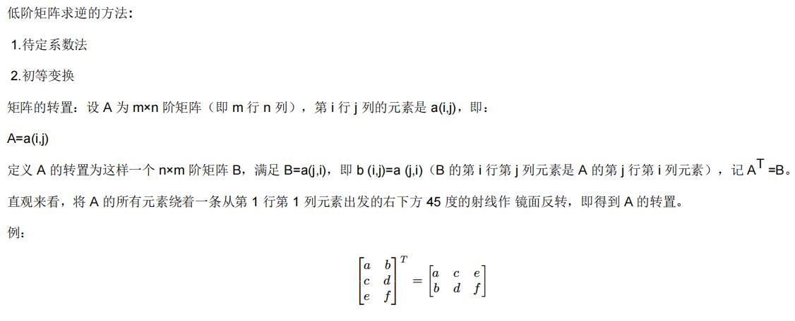
Inverse & transpose

Matrix multiplication

• np.matmul
• np.dot

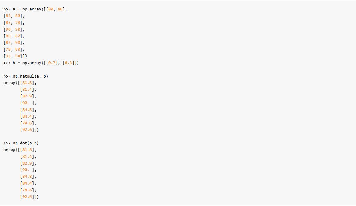
np.matmul and NP Differences between dot:

Both are matrix multiplication. np. Matrix and scalar multiplication are prohibited in matmul. In the inner product operation of vector multiplication vector, NP Matmu and NP Dot makes no difference.

There's a lot of content. I've been sorting it out for a long time. I'm tired.

come on.

thank!

strive!