Two sensor filtering

A car moves in a variable speed straight line with a GPS locator and a speedometer. The data from the two sensors are optimally estimated by Kalman filter. Suppose the observed data is a vector z = [z1 z2] T. z1 is the GPS positioning position and z2 is the speed reading of the speedometer. The covariance matrix R~N(0,R) of Z. The noise of vehicle state equation is wk~N(0,Q). System state matrix A=[1], the predicted value is the previous position, the optimal estimation is the predicted value, plus the difference between the measured value and the predicted value multiplied by the proportion. The calculation formula of Kalman filter is as follows

Optimization: calculate Kk in advance

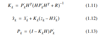
The key to calculate k is the distribution proportion of the measurement difference. k can be calculated through formula (1.11) (1.10) (1.13), and k is only related to the system noise mode Q
It is related to the measurement error covariance matrix R. Therefore, it can be iterated several times in advance to calculate k, but the location estimation can be calculated for a large number of data. Only equations (1.9) and (1.12) need to be calculated. k has been calculated in advance. The five steps of Kalman are simplified to two steps, which greatly reduces the amount of matrix calculation.

Python implementation

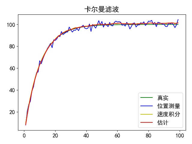
If the true equation of vehicle linear position is 100 *(1 - np.exp(-t/10)), the variance of sensor z1 is 2 and the variance of speedometer z2 is 0.2,
R=[[2 0], system noise variance Q=[1]. System state A=[1], observation matrix H = [1] T
[0 0.2]]

Function pre_kalman, the Kalman filter parameter K can be calculated in advance through the parameter A H Q R_ K. It converges after several iterations.
The function obv() generates the real position of the vehicle according to equation 100 *(1 - np.exp(-t/10)), then adds Gaussian distribution noise respectively, and returns to the sensor for observation
Data z. z0 is GPS position data and z1 is speed. You need to integrate z1 to get the position. Then according to z and k_k for Kalman filter estimation.

Generally, the variance of GPS disturbed position is large and the variance of speedometer is small, but the cumulative error after integration is large. From the figure, the estimated value of Kalman filter fits the real value very well. As shown in the figure

Attached procedure

import numpy as np
import matplotlib
import matplotlib.pyplot as plt
from matplotlib.font_manager import FontProperties

# Preset font
font = {'family': 'SimHei', "size": 14}
matplotlib.rc('font', **font)

'''
Kalman filter, 2-way observation
'''

'''
real
x_k = A*xk_1 + w_k  w_k variance Q
 observation
z_k = H*x_k + v_k   v_k variance R

forecast
x_k_predict = A*x_k_est
p_k_predict = A * p_k_est * A_T + Q
k_k = p_k_predict * H_T *( H*p_k_predict*H_T + R)^-1

Optimal estimation
x_k_est = x_k_predict + k_k *( z_k - H*x_k_predict)
p_k_est = (I - k_k * H) * p_k_predict 
'''

# System status A
A = np.mat([1])

# Observation matrix of two observation instruments
H = np.mat([[1], [1]])

#Observe the instrument variance sigma1 sigma2
sigma1 = 2
sigma2 = 0.2

#System noise wk variance Q
Q = np.mat(1)

'''from Q R count kk'''
def pre_kalman(A,H):
    R=np.mat([[sigma1, 0],[0, sigma2]])
    I=np.mat([1])
    p_est = np.mat([0]) #Estimated covariance matrix
    for _ in np.arange(0,10,1):
        p_predict = A * p_est * A.T + Q #Prediction covariance matrix
        kk = p_predict * H.T * (H * p_predict * H.T + R).I
        p_est = (I - kk * H) * p_predict
    return kk #Return k_k

'''
Two measuring instruments measure two sets of signals,z0 Is the position measurement, z1 Is the speed measurement
z0 The variance of is sigma1,z1 Variance is sigma2
 The true signal is 1-exp(t/10)
'''
def obv():
    t = np.linspace(1,100,100)
    real = 100 *(1 -  np.exp(-t/10))
    #real = t**2

    #Find the speed xdot
    dt = t[1:] - t[:-1]
    dx = real[1:] - real[:-1]
    xdot = dx / dt
    #Fill the 0-th alignment
    xdot = np.hstack([real[0],xdot])

    #Real signal, real noise, error noise of analog measuring instrument
    t = t[:-1]
    real=real[:-1]
    xdot=xdot[:-1]
    z1= real + np.random.normal(0,sigma1,size=t.shape[0])
    z2= xdot + np.random.normal(0,sigma2,size=t.shape[0])
    z = np.mat([(a,b) for (a,b) in zip(z1,z2)])
    return [t, dt, real,z]


'''
Computational Kalman
z Is the observed data
kk Is the Carl slow scale coefficient
'''
def calc_kalman(A,H,z_k,kk):
    global  x_est
    x_pred = A * x_est
    x_est = x_pred + kk * (z_k - H * x_pred)
    return x_est


global x_est #Best estimate
if __name__ == '__main__':

    #Calculate k value
    kk = pre_kalman(A,H)

    #Generate the observation instrument information Z, return time, true value and noisy value of two observation instruments
    [t, dt, xreal, z] = obv()

    x_est=np.mat([0])
    x_est_list=[]

    z1_integral=0
    for k in range(z.shape[0]):
        #Integrate the velocity
        z1_integral += z[k][0,1] * dt[k]
        z[k][0,1] = z1_integral

        #Calculate the Kalman, and the result is in x_est
        calc_kalman(A, H, z[k].T, kk)
        x_est_list.append(x_est[0,0])

    x_est_list=np.array(x_est_list)


    plt.title('Kalman filtering ')
    plt.plot(t, xreal, label='real',color='g')
    plt.plot(t, z[:,0], label='Position measurement',color='b')
    plt.plot(t, z[:,1], label='Velocity integral',color='y')
    plt.plot(t, x_est_list, label='estimate',color='r')
    plt.legend(loc="lower right")
    plt.show()