At present, I am in the third year of junior high school. My ability is limited. If there are deficiencies, I hope to give more advice.

I saw one a week ago video So I want to use python to solve this problem.

○ analysis

Suppose there is a charged particle q in the plane with a mass of m. There is a uniform magnetic field B in space, which is perpendicular to the plane and inward, that is, a gravity field along the negative half axis of the z axis and a gravity field along the negative half axis of the y axis. Charged particles are released from point O in the magnetic field.

The equations of motion of particles can be listed directly

Decompose the equation into x and y directions

The solution of the equations can be obtained simultaneously.

1, dsolve method in Symphony

#Import
from sympy import *
import numpy as np
import matplotlib.pyplot as plt
init_printing()

First declare the symbols x,y,q,m,B,g

#parameter
q,m,B,t,g = symbols('q m B t g',real=True,nonzero=True,positive=True)
#function
x,y = symbols('x y',real=True,nonzero=True,positive=True,cls=Function)

Then express the differential equation

eq1 = Eq(x(t).diff(t,t),-q*B*y(t).diff(t)/m)
eq2 = Eq(y(t).diff(t,t),-g+q*B*x(t).diff(t)/m)
sol = dsolve([eq1,eq2])

Now print out sol (better with Jupiter notebook)

sol

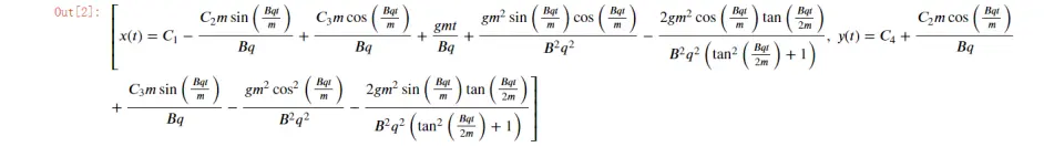
Obviously, this formula is very complicated and simplified by trigsimp()

x = trigsimp(sol[0].rhs)
y = trigsimp(sol[1].rhs)
x,y

Then, you can calculate the integral constant inside

#Define integral variables to avoid error reporting
var('C1 C2 C3 C4')
#x(0)=0
e1 = Eq(x.subs({t:0}),0)
#x'(0)=0, put subs after diff
e2 = Eq(x.diff(t).subs({t:0}),0)
#y(0)=0
e3 = Eq(y.subs({t:0}),0)
#y'(0)=0
e4 = Eq(y.diff(t).subs({t:0}),0)
l = solve([e1,e2,e3,e4],[C1,C2,C3,C4])
l

Then, by substituting the integral constants into x and y, we get the final form of the solution

x = x.subs(l)
y = y.subs(l)
x,y

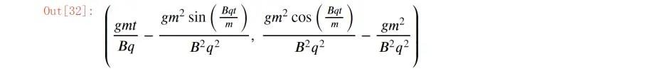
Of course, this solution can also be written in this form

Use plt to draw pictures

ts = np.linspace(0,15,1000)
consts = {q:1,B:1,g:9.8,m:1}
fx = lambdify(t,x.subs(consts),'numpy')
fy = lambdify(t,y.subs(consts),'numpy')
plt.plot(fx(ts),fy(ts))
plt.grid()
plt.show()

But sympy has a disadvantage. When the differential equation is very complex, it will strike directly.

So another new method solved the problem for us

2, SciPy odeint method in integrate

#Import
import numpy as np
from scipy.integrate import odeint
import matplotlib.pyplot as plt
import matplotlib.animation as animation
from math import e

 

We first create a function so that it can represent this differential equation.

For what form this function should have, start with the first-order differential equation

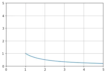
For example, we want to solve the following equation

Its solution is obtained by simply separating variables

Let's solve it with odeint, let y(1)=1

#first order
def f(x,y):
  #The first derivative is expressed as a function of y and x
  dydx = -y/x
  return dydx
#initial condition 
y0 = 1
#The initial value condition is taken at the lower limit of the independent variable x. For example, y(1) will generate a range starting from 1
x = np.linspace(1,5,100)
plt.xlim(0,5)
plt.ylim(0,5)
#For the odeint() method, the tfirst attribute refers to that the first parameter of function f is an argument
sol = odeint(f,y0,x,tfirst=True)
plt.plot(x,sol[:,0])
plt.grid()
plt.show()

Similarly, for the following first-order differential equations

At this point, let's set the vector u=(x,y) (column vector) and turn the system of equations into

In fact, any first-order differential equation can be written in this form

f means

Then the differential equation can be reduced to

And f(t,u) is the function we're looking for

Support vector input in odeint, so this function can be constructed like this

def f(t,u):
  #x1,x2...xn = u
  x,y = u
  #dx1dt=...,dx2dt=...,dxndt=...
  dxdt = 3*x-x*y
  dydt = 2*x-y+e**t
  #dudt = [dx1dt,dx2dt,...dxndt]
  dudt = [dxdt,dydt]
  return dudt
#x1(0)=...,x2(0)=...,xn(0)=...
u0=[0,0]
t = np.linspace(0,10,100)
sol = odeint(f,u0,t,tfirst=True)

Therefore, for second-order ordinary differential equations

We first solve the equation in this form

At this point, this is a system of differential equations about dy/dx and y

Let u=(y,dy/dx), we have

def f(x,u):
	y,dydx = u
	d2ydx2 = np.exp(x)-4*dydx-4*y
	dudx = [dydx,d2ydx2]
	return dudx
u0=[0,0]
x = np.linspace(0,10,100)
sol = odeint(f,u0,x,tfirst=True)

The same is true for higher order differential equations

At this time, we look back at the original problem and can easily get

def f(t,r,k,g):
#k = B*q/m
    x,y,dxdt,dydt = r
    d2xdt2 = -k*dydt
    d2tdt2 = -g + k*dxdt
    return [dxdt,dydt,d2xdt2,d2ydt2]

Define some constants

t = np.linspace(0,15,1000)
k = 1
g = 9.8

Using odeint method

r0 = [0,0,0,0]
sol = odeint(f,r0,t,tfirst = True,args=(k,g))

Draw the image

plt.plot(sol[:,0],sol[:,1])
plt.grid()
plt.show()

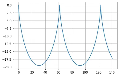
odeint is also very accurate in solving this equation, which is almost the same as sympy.

Finally, we can let him achieve animation effects

def update_points(num):
    point_ani.set_data(s[:,0][num], s[:,1][num])
    return point_ani,
plt.xlabel('X')
plt.ylabel('Y')
fig,ax = plt.subplots()
plt.plot(s[:,0],s[:,1])
point_ani, = plt.plot(s[:,0][0], s[:,1][0], "ro")
plt.grid(ls="--")
# Generate animation
ani = animation.FuncAnimation(fig, update_points,range(1, len(t)), interval=5, blit=True)
plt.show()

If you want to learn more about these two libraries, the official documents are recommended

sympy:https://docs.sympy.org/latest/tutorial/index.html

scipy:https://docs.scipy.org/doc/scipy/reference/tutorial/index.html

I'm going to update several articles recently (if I don't hang up at the end of the term)

Note: I also published this article on site b