Time series analysis
ARIMA
Stationarity: stationarity requires that the fitting curve obtained through the sample time series can continue along the existing form "inertia" in the future
Stationarity requires that the mean and variance of the series do not change significantly
Strict and weak stability:
Yan pingwen: the distribution represented by Yan pingwen does not change with time. For example: white noise (normal), no matter how it is taken, the expectation is 0 and the variance is 1
Weak stationarity: the expectation and correlation coefficient (dependence) remain unchanged. The value Xt of t at a certain time in the future depends on its past information, so dependence is required
Difference method: the difference between time series at time t and time t-1
Autoregressive model (AR)
Describe the relationship between the current value and the historical value, and use the historical time data of the variable to predict itself
The autoregressive model must meet the requirements of stationarity
Formula definition of p-order autoregressive process:
y
t
=
μ
+
∑
i
=
1
p
γ
i
y
t
−
i
+
ϵ
t
y_{t}=\mu+\sum_{i=1}^{p} \gamma_{i} y_{t-i}+\epsilon_{t}
yt=μ+∑i=1pγiyt−i+ϵt
y
t
y_{t}
yt , is the current value
μ
\mu
μ The P-order term is a constant
γ
i
\gamma_{i}
γ i is the autocorrelation coefficient
ϵ
t
\epsilon_{t}
ϵ t is the error
Limitations of autoregressive models
Autoregressive model uses its own data to predict
It must be stable
Must have autocorrelation if autocorrelation coefficient( φ i) Less than 0.5, it should not be used
Autoregression is only applicable to predict the phenomena related to its own early stage
Moving average model (MA)
Moving average model focuses on the accumulation of error terms in autoregressive model
Formula definition of q-order autoregressive process:
y
t
=
μ
+
ϵ
t
+
∑
i
=
1
q
θ
i
ϵ
t
−
i
y_{t}=\mu+\epsilon_{t}+\sum_{i=1}^{q} \theta_{i} \epsilon_{t-i}
yt=μ+ϵt+∑i=1qθiϵt−i
The moving average method can effectively eliminate the random fluctuation in prediction
Autoregressive moving average model (ARMA)
Combination of autoregressive and moving average
Formula definition:
y
t
=
μ
+
∑
i
=
1
p
γ
i
y
t
−
i
+
ϵ
t
+
∑
i
=
1
q
θ
i
ϵ
t
−
i
y_{t}=\mu+\sum_{i=1}^{p} \gamma_{i} y_{t-i}+\epsilon_{t}+\sum_{i=1}^{q} \theta_{i} \epsilon_{t-i}
yt=μ+∑i=1pγiyt−i+ϵt+∑i=1qθiϵt−i
ARIMA(p, d, q) model
The full name is Autoregressive Integrated Moving Average Model (ARIMA)
AR is autoregressive and p is autoregressive term; MA is the moving average, q is the number of moving average items, and d is the number of differences when the time series becomes stationary
Principle: the model is established by transforming non-stationary time series into stationary time series, and then regressing the dependent variable only to its lag value and the present value and lag value of random error term
Autocorrelation function ACF(autocorrelation function)
An ordered sequence of random variables is compared with itself
Autocorrelation function reflects the correlation between the values of the same sequence in different time series
Formula:
A
C
F
(
k
)
=
ρ
k
=
Cov
(
y
t
,
y
t
−
k
)
Var
(
y
t
)
A C F(k)=\rho_{k}=\frac{\operatorname{Cov}\left(y_{t}, y_{t-k}\right)}{\operatorname{Var}\left(y_{t}\right)}
ACF(k)=ρk=Var(yt)Cov(yt,yt−k)
The value range of Pk is [- 1,1]
Partial autocorrelation function (PACF)
For a stationary AR § model, when the autocorrelation coefficient p(k) of lag K is calculated, the simple correlation between x(t) and x(t-k) is not obtained
At the same time, x(t) is also affected by the middle k-1 random variables x(t-1), x(t-2),..., x(t-k+1), and these k-1 random variables are related to x(t-k). Therefore, the autocorrelation coefficient p(k) is actually doped with the influence of other variables on x(t) and x(t-k)
After eliminating the interference of the middle k-1 random variables x(t-1), x(t-2),..., x(t-k+1), the correlation degree of the influence of x(t-k) on x(t).
ACF also includes the influence of other variables, and the partial autocorrelation coefficient PACF is the strict correlation between the two variables
Determination of ARIMA(p, d, q) Order:
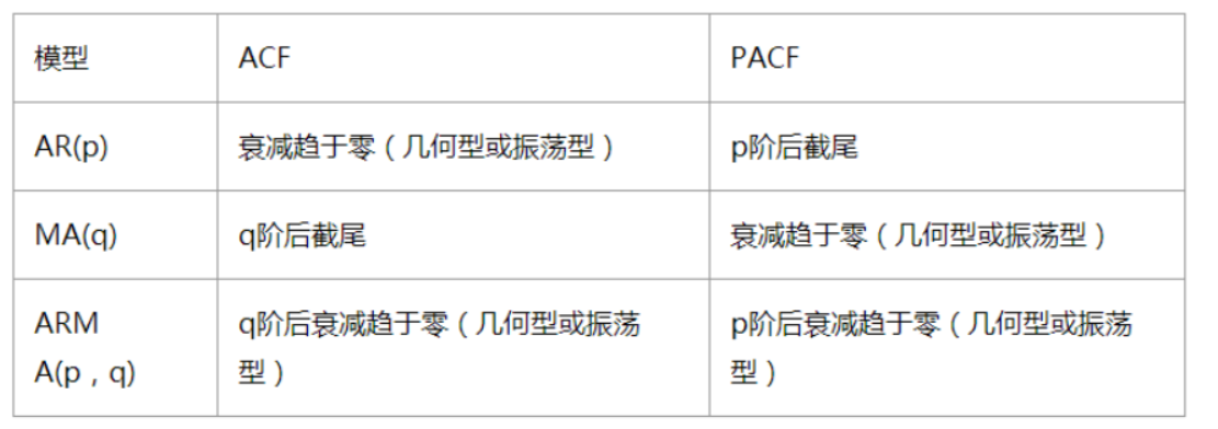
Truncation: falling within the confidence interval (95% of the points comply with the rule)
AR § see PACF; MA(q) looking at ACF
ARIMA modeling process:
Stabilize the sequence (determined by difference method d); Determination of order P and Q: ACF and PACF; ARIMA(p,d,q)
Model selection AIC and BIC: choose a simpler model
AIC: Akaike Information Criterion (AIC)
A
I
C
=
2
k
−
2
ln
(
L
)
A I C=2 k-2 \ln (L)
AIC=2k−2ln(L)
BIC: Bayesian Information Criterion (BIC)
B
I
C
=
k
ln
(
n
)
−
2
ln
(
L
)
B I C=k \ln (n)-2 \ln (L)
BIC=kln(n)−2ln(L)
k is the number of model parameters, n is the number of samples, and L is the likelihood function
Model residual test: whether the residual of ARIMA model is a normal distribution with an average value of 0 and a constant variance
QQ chart: linear or normal distribution
Pandas generate time series
Dates & Times
import pandas as pd
import numpy as np
time series
- timestamp
- Fixed period
- Time interval
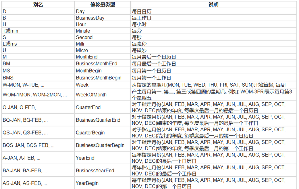
date_range
- You can specify the start time and period
- H: Hours
- D: Oh, my God
- M: Month
# TIMES
#2016 Jul 1; 7/1/2016; 1/7/2016; 2016-07-01; 2016/07/01
# freq refers to frequency, '3D' refers to 3 days
rng = pd.date_range('2016-07-01', periods = 10, freq = '3D')
rng
DatetimeIndex(['2016-07-01', '2016-07-04', '2016-07-07', '2016-07-10',
'2016-07-13', '2016-07-16', '2016-07-19', '2016-07-22',
'2016-07-25', '2016-07-28'],
dtype='datetime64[ns]', freq='3D')
import datetime as dt
time=pd.Series(np.random.randn(20),
           index=pd.date_range(dt.datetime(2016,1,1),periods=20))
print(time)
2016-01-01 -0.188009
2016-01-02 -0.368154
2016-01-03 0.192915
2016-01-04 -1.000698
2016-01-05 -0.324694
2016-01-06 0.570503
2016-01-07 0.014892
2016-01-08 1.441954
2016-01-09 0.768429
2016-01-10 -0.421610
2016-01-11 -0.056000
2016-01-12 0.480678
2016-01-13 1.551418
2016-01-14 0.054797
2016-01-15 0.505593
2016-01-16 -1.217634
2016-01-17 -0.243987
2016-01-18 -1.120619
2016-01-19 -0.492803
2016-01-20 -0.506725
Freq: D, dtype: float64
truncate filtering
time.truncate(before='2016-1-10')
2016-01-10 -0.421610
2016-01-11 -0.056000
2016-01-12 0.480678
2016-01-13 1.551418
2016-01-14 0.054797
2016-01-15 0.505593
2016-01-16 -1.217634
2016-01-17 -0.243987
2016-01-18 -1.120619
2016-01-19 -0.492803
2016-01-20 -0.506725
Freq: D, dtype: float64
time.truncate(after='2016-1-10')
2016-01-01 -0.188009
2016-01-02 -0.368154
2016-01-03 0.192915
2016-01-04 -1.000698
2016-01-05 -0.324694
2016-01-06 0.570503
2016-01-07 0.014892
2016-01-08 1.441954
2016-01-09 0.768429
2016-01-10 -0.421610
Freq: D, dtype: float64
print(time['2016-01-15'])
0.5055933447272851
print(time['2016-01-15':'2016-01-20'])
2016-01-15 0.505593
2016-01-16 -1.217634
2016-01-17 -0.243987
2016-01-18 -1.120619
2016-01-19 -0.492803
2016-01-20 -0.506725
Freq: D, dtype: float64
data=pd.date_range('2010-01-01','2011-01-01',freq='M')
print(data)
DatetimeIndex(['2010-01-31', '2010-02-28', '2010-03-31', '2010-04-30',
'2010-05-31', '2010-06-30', '2010-07-31', '2010-08-31',
'2010-09-30', '2010-10-31', '2010-11-30', '2010-12-31'],
dtype='datetime64[ns]', freq='M')
#time stamp
pd.Timestamp('2016-07-10')
Timestamp('2016-07-10 00:00:00')
# You can specify more details
pd.Timestamp('2016-07-10 10')
Timestamp('2016-07-10 10:00:00')
pd.Timestamp('2016-07-10 10:15')
Timestamp('2016-07-10 10:15:00')
t = pd.Timestamp('2016-07-10 10:15')
# Time interval
pd.Period('2016-01')
Period('2016-01', 'M')
pd.Period('2016-01-01')
Period('2016-01-01', 'D')
# TIME OFFSETS
# Time addition and subtraction
pd.Timedelta('1 day')
Timedelta('1 days 00:00:00')
pd.Period('2016-01-01 10:10') + pd.Timedelta('1 day')
Period('2016-01-02 10:10', 'T')
pd.Timestamp('2016-01-01 10:10') + pd.Timedelta('1 day')
Timestamp('2016-01-02 10:10:00')
pd.Timestamp('2016-01-01 10:10') + pd.Timedelta('15 ns')
Timestamp('2016-01-01 10:10:00.000000015')
p1 = pd.period_range('2016-01-01 10:10', freq = '25H', periods = 10)
p2 = pd.period_range('2016-01-01 10:10', freq = '1D1H', periods = 10)
p1
PeriodIndex(['2016-01-01 10:00', '2016-01-02 11:00', '2016-01-03 12:00',
'2016-01-04 13:00', '2016-01-05 14:00', '2016-01-06 15:00',
'2016-01-07 16:00', '2016-01-08 17:00', '2016-01-09 18:00',
'2016-01-10 19:00'],
dtype='period[25H]')
p2
PeriodIndex(['2016-01-01 10:00', '2016-01-02 11:00', '2016-01-03 12:00',
'2016-01-04 13:00', '2016-01-05 14:00', '2016-01-06 15:00',
'2016-01-07 16:00', '2016-01-08 17:00', '2016-01-09 18:00',
'2016-01-10 19:00'],
dtype='period[25H]')
# Specify index
rng = pd.date_range('2016 Jul 1', periods = 10, freq = 'D')
rng
pd.Series(range(len(rng)), index = rng)
2016-07-01 0
2016-07-02 1
2016-07-03 2
2016-07-04 3
2016-07-05 4
2016-07-06 5
2016-07-07 6
2016-07-08 7
2016-07-09 8
2016-07-10 9
Freq: D, dtype: int64
periods = [pd.Period('2016-01'), pd.Period('2016-02'), pd.Period('2016-03')]
ts = pd.Series(np.random.randn(len(periods)), index = periods)
ts
2016-01 0.340616
2016-02 0.255040
2016-03 -1.991041
Freq: M, dtype: float64
type(ts.index)
# Timestamps and time periods can be converted
ts = pd.Series(range(10), pd.date_range('07-10-16 8:00', periods = 10, freq = 'H'))
ts
2016-07-10 08:00:00 0
2016-07-10 09:00:00 1
2016-07-10 10:00:00 2
2016-07-10 11:00:00 3
2016-07-10 12:00:00 4
2016-07-10 13:00:00 5
2016-07-10 14:00:00 6
2016-07-10 15:00:00 7
2016-07-10 16:00:00 8
2016-07-10 17:00:00 9
Freq: H, dtype: int64
ts_period = ts.to_period()
ts_period
2016-07-10 08:00 0
2016-07-10 09:00 1
2016-07-10 10:00 2
2016-07-10 11:00 3
2016-07-10 12:00 4
2016-07-10 13:00 5
2016-07-10 14:00 6
2016-07-10 15:00 7
2016-07-10 16:00 8
2016-07-10 17:00 9
Freq: H, dtype: int64
ts_period['2016-07-10 08:30':'2016-07-10 11:45']
2016-07-10 08:00 0
2016-07-10 09:00 1
2016-07-10 10:00 2
2016-07-10 11:00 3
Freq: H, dtype: int64
ts['2016-07-10 08:30':'2016-07-10 11:45']
2016-07-10 09:00:00 1
2016-07-10 10:00:00 2
2016-07-10 11:00:00 3
Freq: H, dtype: int64
Pandas data resampling
import pandas as pd
import numpy as np
Data resampling
- Time data is converted from one frequency to another
- Downsampling
- Liter sampling
rng = pd.date_range('1/1/2011', periods=90, freq='D')
ts = pd.Series(np.random.randn(len(rng)), index=rng)
ts.head()
2011-01-01 1.325061
2011-01-02 -0.007781
2011-01-03 -0.574297
2011-01-04 1.179030
2011-01-05 -1.892891
Freq: D, dtype: float64
ts.resample('M').sum()
2011-01-31 7.061535
2011-02-28 -1.360312
2011-03-31 -4.334479
Freq: M, dtype: float64
ts.resample('3D').sum()
2011-01-01 0.742984
2011-01-04 1.168289
2011-01-07 -2.558146
2011-01-10 -0.596113
2011-01-13 -0.822468
2011-01-16 1.264703
2011-01-19 3.908058
2011-01-22 2.020699
2011-01-25 1.829759
2011-01-28 -0.606650
2011-01-31 1.142033
2011-02-03 1.605801
2011-02-06 -2.059437
2011-02-09 -0.432942
2011-02-12 0.403229
2011-02-15 2.503971
2011-02-18 1.992525
2011-02-21 -1.553652
2011-02-24 -1.669596
2011-02-27 -1.248293
2011-03-02 -5.028106
2011-03-05 -0.501333
2011-03-08 0.694710
2011-03-11 -1.223193
2011-03-14 -1.395738
2011-03-17 -0.689522
2011-03-20 2.783964
2011-03-23 0.465247
2011-03-26 -0.812388
2011-03-29 0.038350
Freq: 3D, dtype: float64
day3Ts = ts.resample('3D').mean()
day3Ts
2011-01-01 0.247661
2011-01-04 0.389430
2011-01-07 -0.852715
2011-01-10 -0.198704
2011-01-13 -0.274156
2011-01-16 0.421568
2011-01-19 1.302686
2011-01-22 0.673566
2011-01-25 0.609920
2011-01-28 -0.202217
2011-01-31 0.380678
2011-02-03 0.535267
2011-02-06 -0.686479
2011-02-09 -0.144314
2011-02-12 0.134410
2011-02-15 0.834657
2011-02-18 0.664175
2011-02-21 -0.517884
2011-02-24 -0.556532
2011-02-27 -0.416098
2011-03-02 -1.676035
2011-03-05 -0.167111
2011-03-08 0.231570
2011-03-11 -0.407731
2011-03-14 -0.465246
2011-03-17 -0.229841
2011-03-20 0.927988
2011-03-23 0.155082
2011-03-26 -0.270796
2011-03-29 0.012783
Freq: 3D, dtype: float64
print(day3Ts.resample('D').asfreq())
2011-01-01 0.247661
2011-01-02 NaN
2011-01-03 NaN
2011-01-04 0.389430
2011-01-05 NaN
...
2011-03-25 NaN
2011-03-26 -0.270796
2011-03-27 NaN
2011-03-28 NaN
2011-03-29 0.012783
Freq: D, Length: 88, dtype: float64
Interpolation method:
- Fill null value takes the previous value
- bfill null value takes the following value
- interpolate linear value
day3Ts.resample('D').ffill(1)
2011-01-01 0.247661
2011-01-02 0.247661
2011-01-03 NaN
2011-01-04 0.389430
2011-01-05 0.389430
...
2011-03-25 NaN
2011-03-26 -0.270796
2011-03-27 -0.270796
2011-03-28 NaN
2011-03-29 0.012783
Freq: D, Length: 88, dtype: float64
day3Ts.resample('D').bfill(1)
2011-01-01 0.247661
2011-01-02 NaN
2011-01-03 0.389430
2011-01-04 0.389430
2011-01-05 NaN
...
2011-03-25 -0.270796
2011-03-26 -0.270796
2011-03-27 NaN
2011-03-28 0.012783
2011-03-29 0.012783
Freq: D, Length: 88, dtype: float64
day3Ts.resample('D').interpolate('linear')
2011-01-01 0.247661
2011-01-02 0.294917
2011-01-03 0.342174
2011-01-04 0.389430
2011-01-05 -0.024619
...
2011-03-25 -0.128836
2011-03-26 -0.270796
2011-03-27 -0.176269
2011-03-28 -0.081743
2011-03-29 0.012783
Freq: D, Length: 88, dtype: float64
Pandas sliding window
%matplotlib inline
import matplotlib.pylab
import numpy as np
import pandas as pd
df = pd.Series(np.random.randn(600), index = pd.date_range('7/1/2016', freq = 'D', periods = 600))
df.head()
2016-07-01 1.427084
2016-07-02 0.074392
2016-07-03 -0.806538
2016-07-04 0.973909
2016-07-05 -0.196484
Freq: D, dtype: float64
r = df.rolling(window = 10)
r
Rolling [window=10,center=False,axis=0,method=single]
#r.max, r.median, r.std, r.skew, r.sum, r.var
print(r.mean())
2016-07-01 NaN
2016-07-02 NaN
2016-07-03 NaN
2016-07-04 NaN
2016-07-05 NaN
...
2018-02-16 -0.044556
2018-02-17 -0.172443
2018-02-18 -0.247636
2018-02-19 -0.109076
2018-02-20 -0.159144
Freq: D, Length: 600, dtype: float64
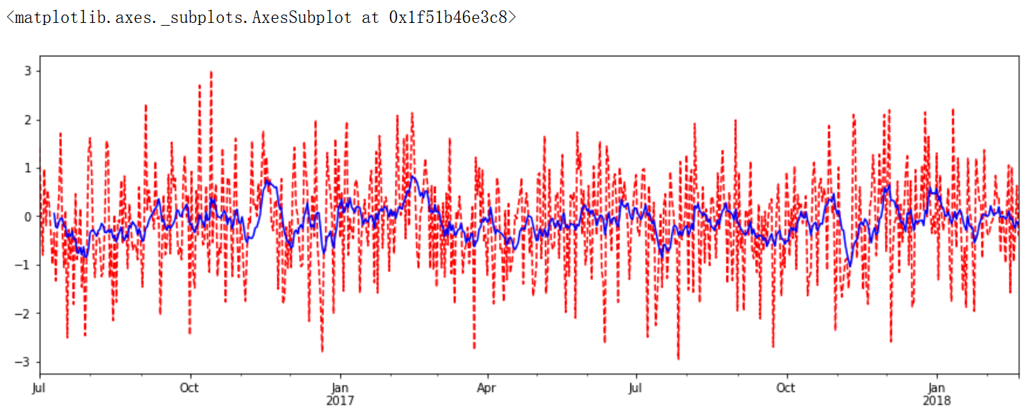
import matplotlib.pyplot as plt
%matplotlib inline

plt.figure(figsize=(15, 5))

df.plot(style='r--')
df.rolling(window=10).mean().plot(style='b')
ARIMA model example
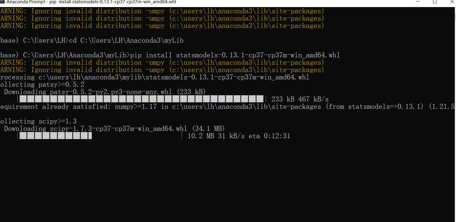
Download statsmodels Library
If you directly pip, it will be very slow and the network is easy to break, which is very annoying. It is suggested to go to this website: https://www.lfd.uci.edu/ ~Gohlke / Python LIBS /, Search Stats models, download the corresponding version, and then download the library from the local pip, but it's still a little slow.
Establish ARIMA model
# http://www.lfd.uci.edu/~gohlke/pythonlibs / Library Download Website
from __future__ import absolute_import, division, print_function
%load_ext autoreload
%autoreload 2
%matplotlib inline
%config InlineBackend.figure_format='retina'


import sys
import os

import pandas as pd
import numpy as np

# # Remote Data Access
# import pandas_datareader.data as web
# import datetime
# # reference: https://pandas-datareader.readthedocs.io/en/latest/remote_data.html

# TSA from Statsmodels
import statsmodels.api as sm
import statsmodels.formula.api as smf
import statsmodels.tsa.api as smt

# Display and Plotting
import matplotlib.pylab as plt
import seaborn as sns

pd.set_option('display.float_format', lambda x: '%.5f' % x) # pandas
np.set_printoptions(precision=5, suppress=True) # numpy

pd.set_option('display.max_columns', 100)
pd.set_option('display.max_rows', 100)

# seaborn plotting style
sns.set(style='ticks', context='poster')
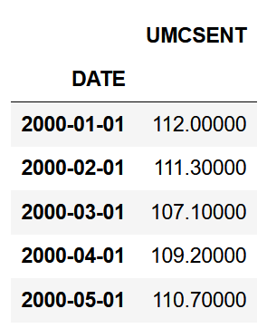
#Read the data
#US consumer confidence index
Sentiment = 'data/sentiment.csv'
Sentiment = pd.read_csv(Sentiment, index_col=0, parse_dates=[0])
Sentiment.head()
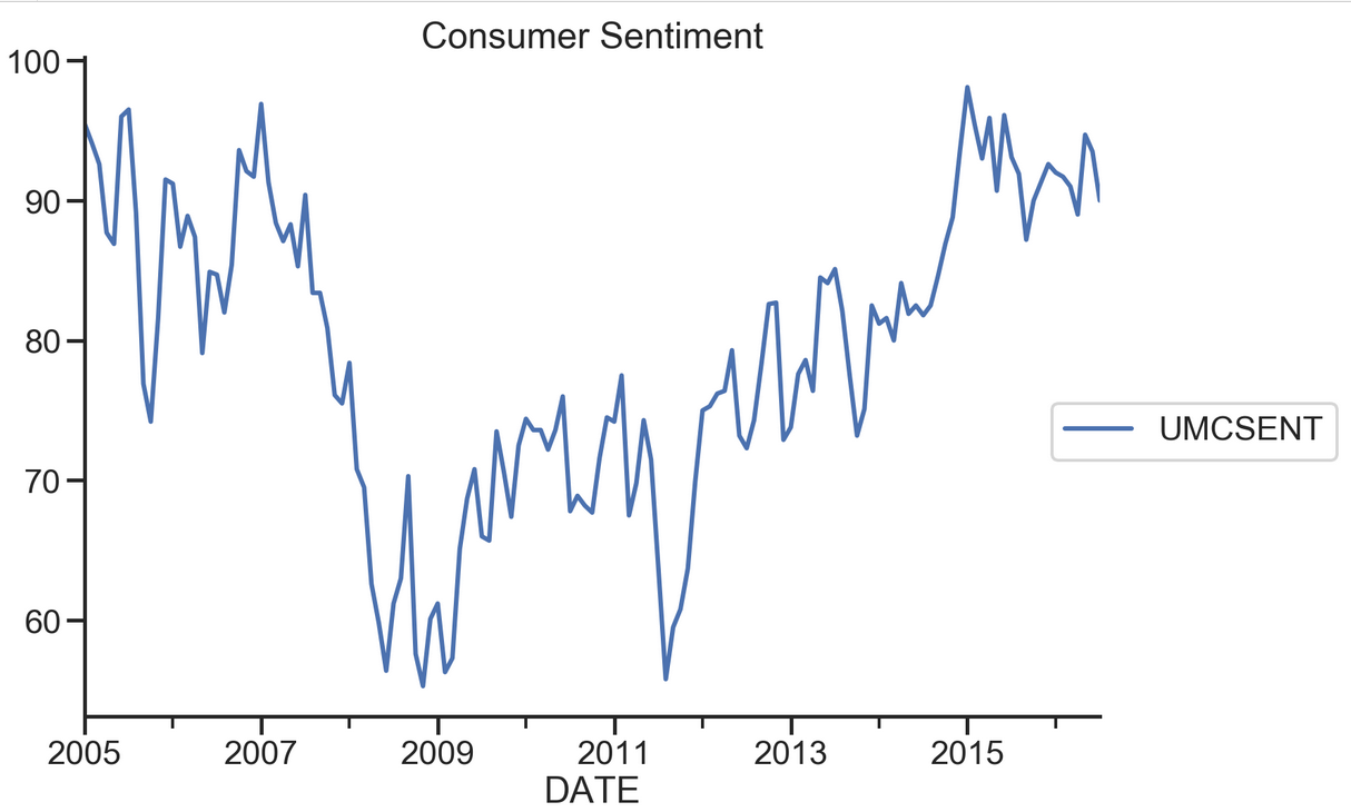
# Select the series from 2005 - 2016
sentiment_short = Sentiment.loc['2005':'2016']
sentiment_short.plot(figsize=(12,8))
plt.legend(bbox_to_anchor=(1.25, 0.5))
plt.title("Consumer Sentiment")
sns.despine()
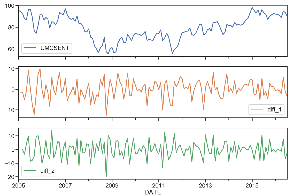
sentiment_short['diff_1'] = sentiment_short['UMCSENT'].diff(1)

sentiment_short['diff_2'] = sentiment_short['diff_1'].diff(1)

sentiment_short.plot(subplots=True, figsize=(18, 12))
del sentiment_short['diff_2']
del sentiment_short['diff_1']
sentiment_short.head()
print (type(sentiment_short))
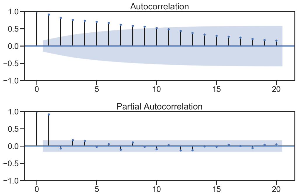
fig = plt.figure(figsize=(12,8))

ax1 = fig.add_subplot(211)
fig = sm.graphics.tsa.plot_acf(sentiment_short, lags=20,ax=ax1)
ax1.xaxis.set_ticks_position('bottom')
fig.tight_layout();

ax2 = fig.add_subplot(212)
fig = sm.graphics.tsa.plot_pacf(sentiment_short, lags=20, ax=ax2)
ax2.xaxis.set_ticks_position('bottom')
fig.tight_layout();
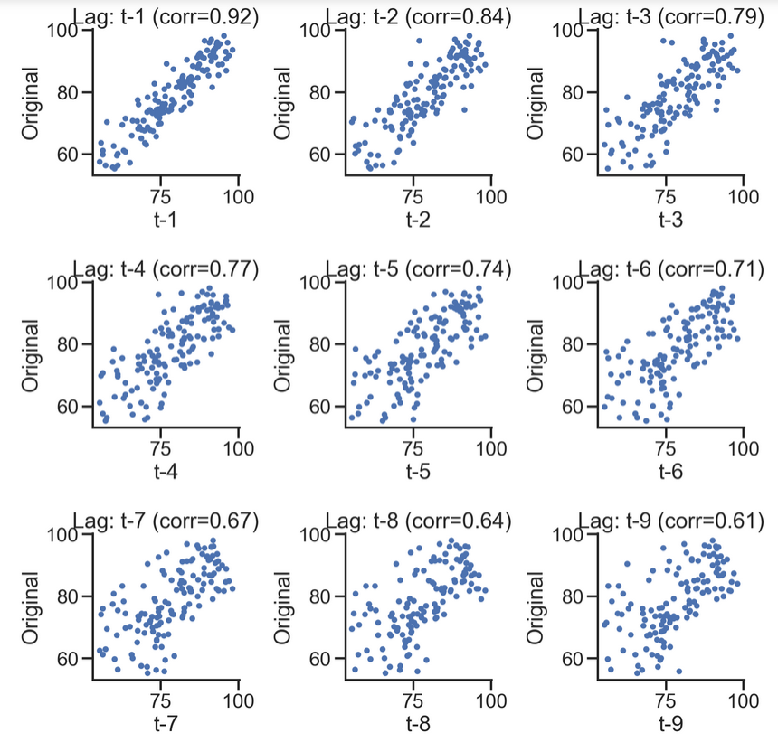
# Scatter diagrams can also represent

lags=9

ncols=3
nrows=int(np.ceil(lags/ncols))

fig, axes = plt.subplots(ncols=ncols, nrows=nrows, figsize=(4*ncols, 4*nrows))

for ax, lag in zip(axes.flat, np.arange(1,lags+1, 1)):
    lag_str = 't-{}'.format(lag)
    X = (pd.concat([sentiment_short, sentiment_short.shift(-lag)], axis=1,
                   keys=['y'] + [lag_str]).dropna())

    X.plot(ax=ax, kind='scatter', y='y', x=lag_str);
    corr = X.corr().iloc[:,:].values[0][1]
    ax.set_ylabel('Original')
    ax.set_title('Lag: {} (corr={:.2f})'.format(lag_str, corr));
    ax.set_aspect('equal');
    sns.despine();

fig.tight_layout();
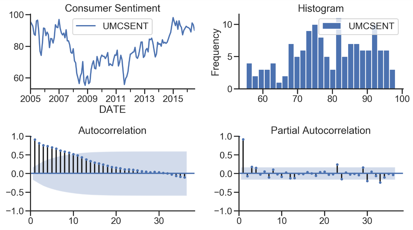
# More intuitive

def tsplot(y, lags=None, title='', figsize=(14, 8)):

    fig = plt.figure(figsize=figsize)
    layout = (2, 2)
    ts_ax   = plt.subplot2grid(layout, (0, 0))
    hist_ax = plt.subplot2grid(layout, (0, 1))
    acf_ax  = plt.subplot2grid(layout, (1, 0))
    pacf_ax = plt.subplot2grid(layout, (1, 1))

    y.plot(ax=ts_ax)
    ts_ax.set_title(title)
    y.plot(ax=hist_ax, kind='hist', bins=25)
    hist_ax.set_title('Histogram')
    smt.graphics.plot_acf(y, lags=lags, ax=acf_ax)
    smt.graphics.plot_pacf(y, lags=lags, ax=pacf_ax)
    [ax.set_xlim(0) for ax in [acf_ax, pacf_ax]]
    sns.despine()
    plt.tight_layout()
    return ts_ax, acf_ax, pacf_ax
tsplot(sentiment_short, title='Consumer Sentiment', lags=36);
Parameter selection
from __future__ import absolute_import, division, print_function
%load_ext autoreload
%autoreload 2
%matplotlib inline
%config InlineBackend.figure_format='retina'


import sys
import os

import pandas as pd
import numpy as np

# TSA from Statsmodels
import statsmodels.api as sm
import statsmodels.formula.api as smf
import statsmodels.tsa.api as smt

# Display and Plotting
import matplotlib.pylab as plt
import seaborn as sns

pd.set_option('display.float_format', lambda x: '%.5f' % x) # pandas
np.set_printoptions(precision=5, suppress=True) # numpy

pd.set_option('display.max_columns', 100)
pd.set_option('display.max_rows', 100)

# seaborn plotting style
sns.set(style='ticks', context='poster')
filename_ts = 'data/series1.csv'
ts_df = pd.read_csv(filename_ts, index_col=0, parse_dates=[0])

n_sample = ts_df.shape[0]
print(ts_df.shape)
print(ts_df.head())
(120, 1)
value
2006-06-01 0.21507
2006-07-01 1.14225
2006-08-01 0.08077
2006-09-01 -0.73952
2006-10-01 0.53552
# Create a training sample and testing sample before analyzing the series

n_train=int(0.95*n_sample)+1
n_forecast=n_sample-n_train
#ts_df
ts_train = ts_df.iloc[:n_train]['value']
ts_test = ts_df.iloc[n_train:]['value']
print(ts_train.shape)
print(ts_test.shape)
print("Training Series:", "\n", ts_train.tail(), "\n")
print("Testing Series:", "\n", ts_test.head())
(115,)
(5,)
Training Series:
2015-08-01 0.60371
2015-09-01 -1.27372
2015-10-01 -0.93284
2015-11-01 0.08552
2015-12-01 1.20534
Name: value, dtype: float64
Testing Series:
2016-01-01 2.16411
2016-02-01 0.95226
2016-03-01 0.36485
2016-04-01 -2.26487
2016-05-01 -2.38168
Name: value, dtype: float64
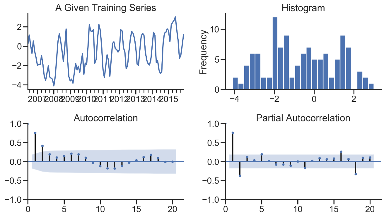
def tsplot(y, lags=None, title='', figsize=(14, 8)):

    fig = plt.figure(figsize=figsize)
    layout = (2, 2)
    ts_ax   = plt.subplot2grid(layout, (0, 0))
    hist_ax = plt.subplot2grid(layout, (0, 1))
    acf_ax  = plt.subplot2grid(layout, (1, 0))
    pacf_ax = plt.subplot2grid(layout, (1, 1))

    y.plot(ax=ts_ax)
    ts_ax.set_title(title)
    y.plot(ax=hist_ax, kind='hist', bins=25)
    hist_ax.set_title('Histogram')
    smt.graphics.plot_acf(y, lags=lags, ax=acf_ax)
    smt.graphics.plot_pacf(y, lags=lags, ax=pacf_ax)
    [ax.set_xlim(0) for ax in [acf_ax, pacf_ax]]
    sns.despine()
    fig.tight_layout()
    return ts_ax, acf_ax, pacf_ax
tsplot(ts_train, title='A Given Training Series', lags=20);
#Model Estimation

# Fit the model
arima200 = sm.tsa.SARIMAX(ts_train, order=(2,0,0))
model_results = arima200.fit()
import itertools

p_min = 0
d_min = 0
q_min = 0
p_max = 4
d_max = 0
q_max = 4

# Initialize a DataFrame to store the results
results_bic = pd.DataFrame(index=['AR{}'.format(i) for i in range(p_min,p_max+1)],
                           columns=['MA{}'.format(i) for i in range(q_min,q_max+1)])

for p,d,q in itertools.product(range(p_min,p_max+1),
                               range(d_min,d_max+1),
                               range(q_min,q_max+1)):
    if p==0 and d==0 and q==0:
        results_bic.loc['AR{}'.format(p), 'MA{}'.format(q)] = np.nan
        continue

    try:
        model = sm.tsa.SARIMAX(ts_train, order=(p, d, q),
                               #enforce_stationarity=False,
                               #enforce_invertibility=False,
                              )
        results = model.fit()
        results_bic.loc['AR{}'.format(p), 'MA{}'.format(q)] = results.bic
    except:
        continue
results_bic = results_bic[results_bic.columns].astype(float)
fig, ax = plt.subplots(figsize=(10, 8))
ax = sns.heatmap(results_bic,
                 mask=results_bic.isnull(),
                 ax=ax,
                 annot=True,
                 fmt='.2f',
                 );
ax.set_title('BIC');
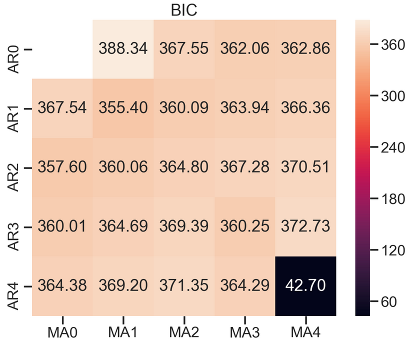
# Alternative model selection method, limited to only searching AR and MA parameters

train_results = sm.tsa.arma_order_select_ic(ts_train, ic=['aic', 'bic'], trend='n', max_ar=4, max_ma=4)

print('AIC', train_results.aic_min_order)
print('BIC', train_results.bic_min_order)
AIC (4, 4)
BIC (4, 4)
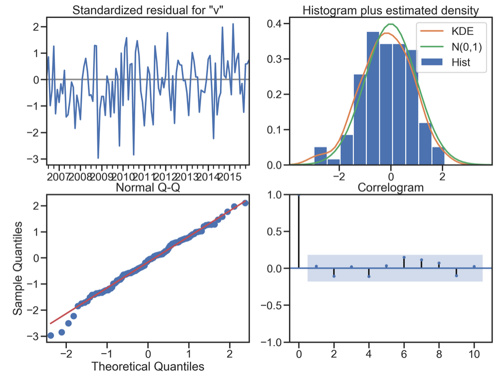
#Residual analysis normal distribution QQ linear graph
model_results.plot_diagnostics(figsize=(16, 12));
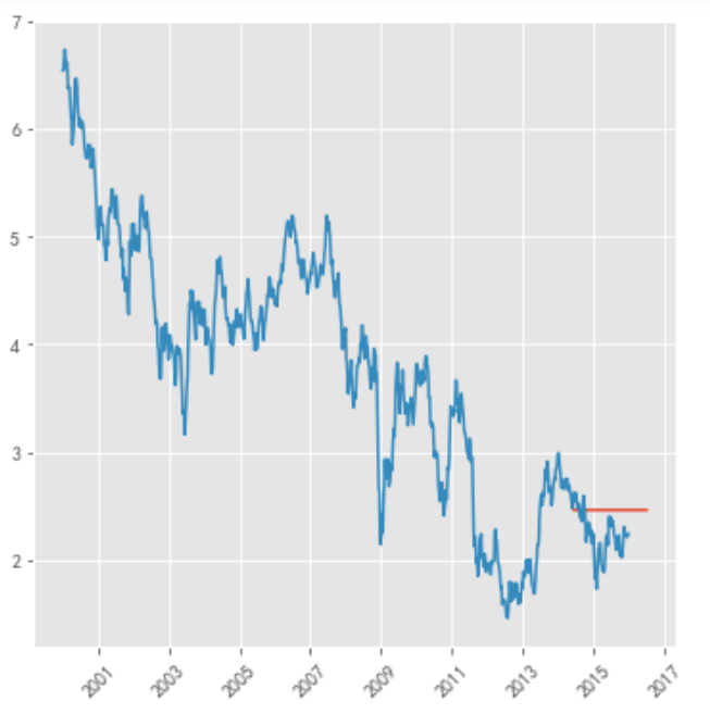
Time series prediction with ARIMA model - stock prediction
%matplotlib inline
import pandas as pd
import pandas_datareader
import datetime
import matplotlib.pylab as plt
import seaborn as sns
from matplotlib.pylab import style
# from statsmodels.tsa.arima_model import ARIMA
from statsmodels.graphics.tsaplots import plot_acf, plot_pacf

style.use('ggplot')
plt.rcParams['font.sans-serif'] = ['SimHei']
plt.rcParams['axes.unicode_minus'] = False
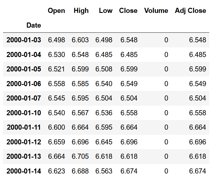
stockFile = 'data/T10yr.csv'
stock = pd.read_csv(stockFile, index_col=0, parse_dates=[0])
stock.head(10)
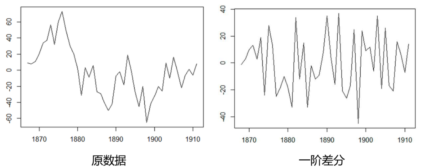
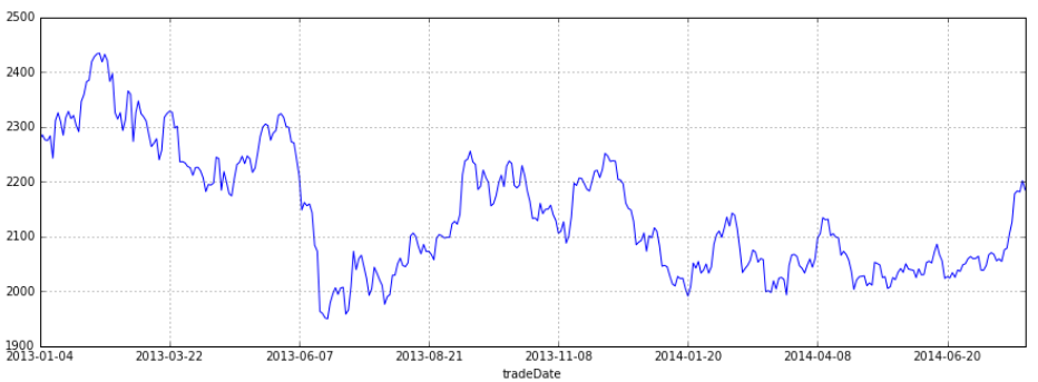
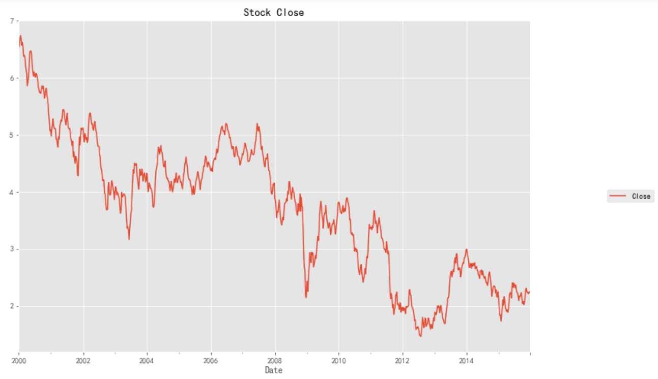
stock_week = stock['Close'].resample('W-MON').mean()
stock_train = stock_week['2000':'2015']
stock_train.plot(figsize=(12,8))
plt.legend(bbox_to_anchor=(1.25, 0.5))
plt.title("Stock Close")
sns.despine()
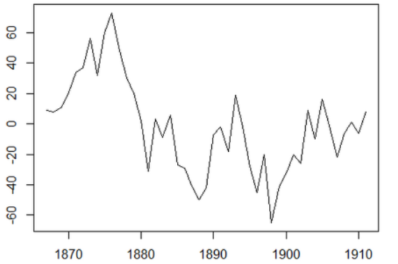
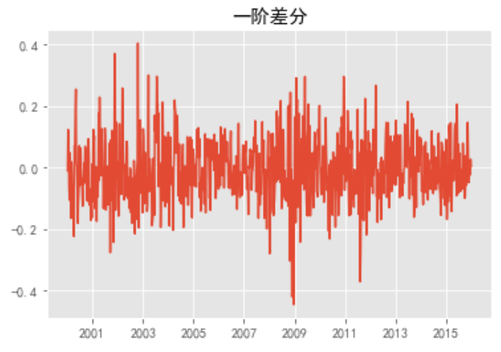
stock_diff = stock_train.diff()
stock_diff = stock_diff.dropna()

plt.figure()
plt.plot(stock_diff)
plt.title('First order difference')
plt.show()
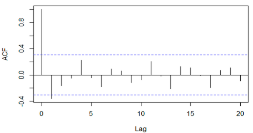
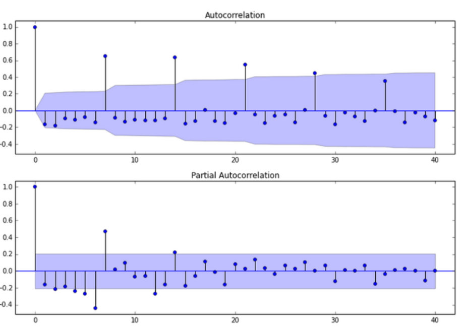
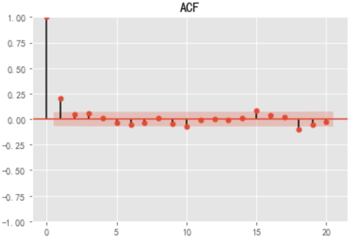
acf = plot_acf(stock_diff, lags=20)
plt.title("ACF")
acf.show()
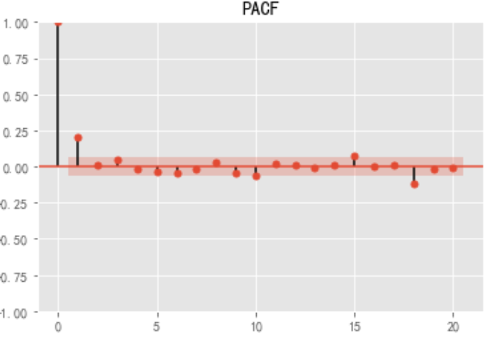
pacf = plot_pacf(stock_diff, lags=20)
plt.title("PACF")
pacf.show()
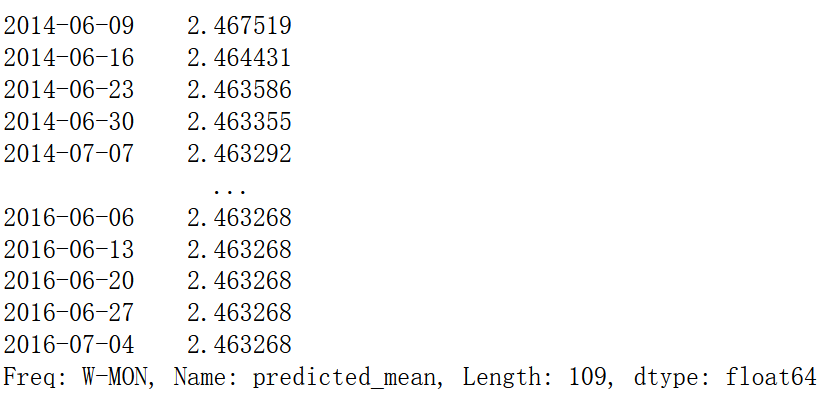
import statsmodels.api as sm
model = sm.tsa.arima.ARIMA(stock_train, order=(1, 1, 1),freq='W-MON')
result = model.fit()
#print(result.summary())
pred = result.predict('20140609', '20160701',dynamic=True, typ='levels')
print (pred)
plt.figure(figsize=(6, 6))
plt.xticks(rotation=45)
plt.plot(pred)
plt.plot(stock_train)
Use tsfresh library for classification tasks
Problems encountered installing tsfresh
I really took it. There was no tsfresh library on that website, so I had to pip install tsfresh, but there was an error. I don't know why the installation failed. Then I reinstalled and encountered some problems,
1. To solve the problem that "llvmlite" cannot be installed and uninstalled, you need to go to anaconda3 → Lib → site packages, find the corresponding old version file, and delete it directly. (the following is what I deleted)

Reference blog https://blog.csdn.net/wasjrong/article/details/108419050
2 is an ERROR: Could not install packages due to an EnvironmentError: [WinError 5] access is denied. You need to add -- user + the name of the package to be installed after pip install, for example
pip install --user tsfresh
Sometimes I really hate direct pip install. I really hope the library website can collect more libraries, so there won't be so many problems when downloading.
test
%matplotlib inline
import matplotlib.pylab as plt
import seaborn as sns
from tsfresh.examples.robot_execution_failures import download_robot_execution_failures, load_robot_execution_failures
from tsfresh import extract_features, extract_relevant_features, select_features
from tsfresh.utilities.dataframe_functions import impute
from tsfresh.feature_extraction import ComprehensiveFCParameters
from sklearn.tree import DecisionTreeClassifier
from sklearn.model_selection import train_test_split
from sklearn.metrics import classification_report


#http://tsfresh.readthedocs.io/en/latest/text/quick_start.html Document introduction
# An error ConnectionError will be reported here:
# Reference articles https://blog.csdn.net/The_Time_Runner/article/details/110248835
download_robot_execution_failures()
df, y = load_robot_execution_failures()
df.head()
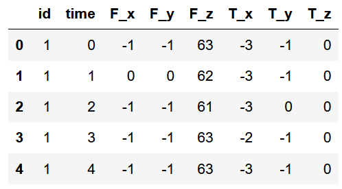
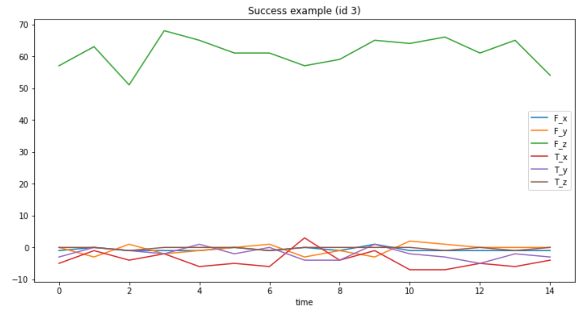
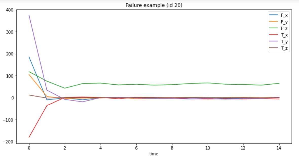
df[df.id == 3][['time', 'F_x', 'F_y', 'F_z', 'T_x', 'T_y', 'T_z']].plot(x='time', title='Success example (id 3)', figsize=(12, 6));
df[df.id == 20][['time', 'F_x', 'F_y', 'F_z', 'T_x', 'T_y', 'T_z']].plot(x='time', title='Failure example (id 20)', figsize=(12, 6));
extraction_settings = ComprehensiveFCParameters()
#column_id (str) – The name of the id column to group by
#column_sort (str) – The name of the sort column.
X = extract_features(df,
                     column_id='id', column_sort='time',
                     default_fc_parameters=extraction_settings,
                     impute_function= impute)
X.head()
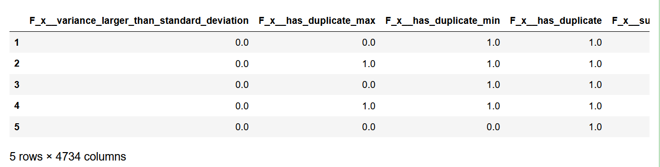
X.info()
<class 'pandas.core.frame.DataFrame'>
Int64Index: 88 entries, 1 to 88
Columns: 4734 entries, F_x__variance_larger_than_standard_deviation to T_z__mean_n_absolute_max__number_of_maxima_7
dtypes: float64(4734)
memory usage: 3.2 MB
X_filtered = extract_relevant_features(df, y,
                                       column_id='id', column_sort='time',
                                       default_fc_parameters=extraction_settings)
X_filtered.head()
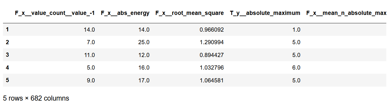
X_filtered.info()
<class 'pandas.core.frame.DataFrame'>
Int64Index: 88 entries, 1 to 88
Columns: 682 entries, F_x__value_count__value_-1 to T_z__quantile__q_0.9
dtypes: float64(682)
memory usage: 469.6 KB
X_train, X_test, X_filtered_train, X_filtered_test, y_train, y_test = train_test_split(X, X_filtered, y, test_size=.4)
cl = DecisionTreeClassifier()
cl.fit(X_train, y_train)
print(classification_report(y_test, cl.predict(X_test)))
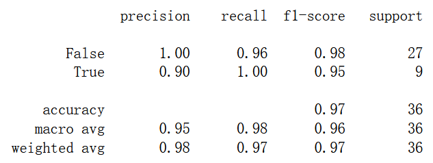
cl.n_features_
4734
cl2 = DecisionTreeClassifier()
cl2.fit(X_filtered_train, y_train)
print(classification_report(y_test, cl2.predict(X_filtered_test)))
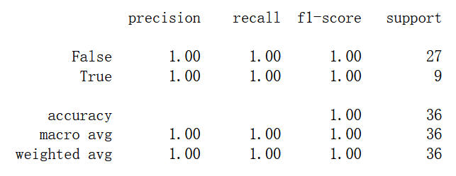
cl2.n_features_
682
Wikipedia entry EDA
import pandas as pd
import numpy as np
import matplotlib.pyplot as plt
import re
%matplotlib inline
train = pd.read_csv('train_1.csv').fillna(0)
train.head()
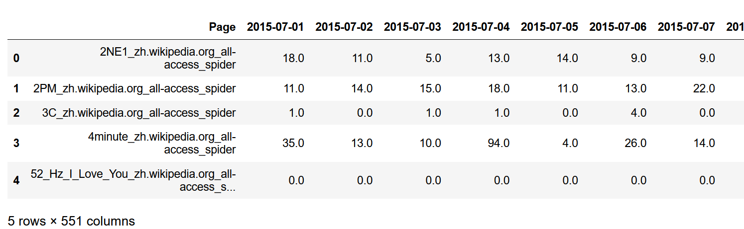
train.info()
<class 'pandas.core.frame.DataFrame'>
RangeIndex: 145063 entries, 0 to 145062
Columns: 551 entries, Page to 2016-12-31
dtypes: float64(550), object(1)
memory usage: 609.8+ MB
for col in train.columns[1:]:
    train[col] = pd.to_numeric(train[col],downcast='integer')
train.head()
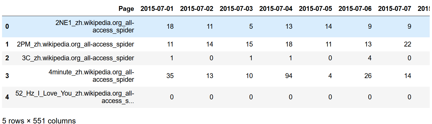
train.info()
<class 'pandas.core.frame.DataFrame'>
RangeIndex: 145063 entries, 0 to 145062
Columns: 551 entries, Page to 2016-12-31
dtypes: int32(550), object(1)
memory usage: 305.5+ MB
def get_language(page):
    res = re.search('[a-z][a-z].wikipedia.org',page)
    #print (res.group()[0:2])
    if res:
        return res.group()[0:2]
    return 'na'

train['lang'] = train.Page.map(get_language)

from collections import Counter

print(Counter(train.lang))
Counter({'en': 24108, 'ja': 20431, 'de': 18547, 'na': 17855, 'fr': 17802, 'zh': 17229, 'ru': 15022, 'es': 14069})
lang_sets = {}
lang_sets['en'] = train[train.lang=='en'].iloc[:,0:-1]
lang_sets['ja'] = train[train.lang=='ja'].iloc[:,0:-1]
lang_sets['de'] = train[train.lang=='de'].iloc[:,0:-1]
lang_sets['na'] = train[train.lang=='na'].iloc[:,0:-1]
lang_sets['fr'] = train[train.lang=='fr'].iloc[:,0:-1]
lang_sets['zh'] = train[train.lang=='zh'].iloc[:,0:-1]
lang_sets['ru'] = train[train.lang=='ru'].iloc[:,0:-1]
lang_sets['es'] = train[train.lang=='es'].iloc[:,0:-1]

sums = {}
for key in lang_sets:
    sums[key] = lang_sets[key].iloc[:,1:].sum(axis=0) / lang_sets[key].shape[0]
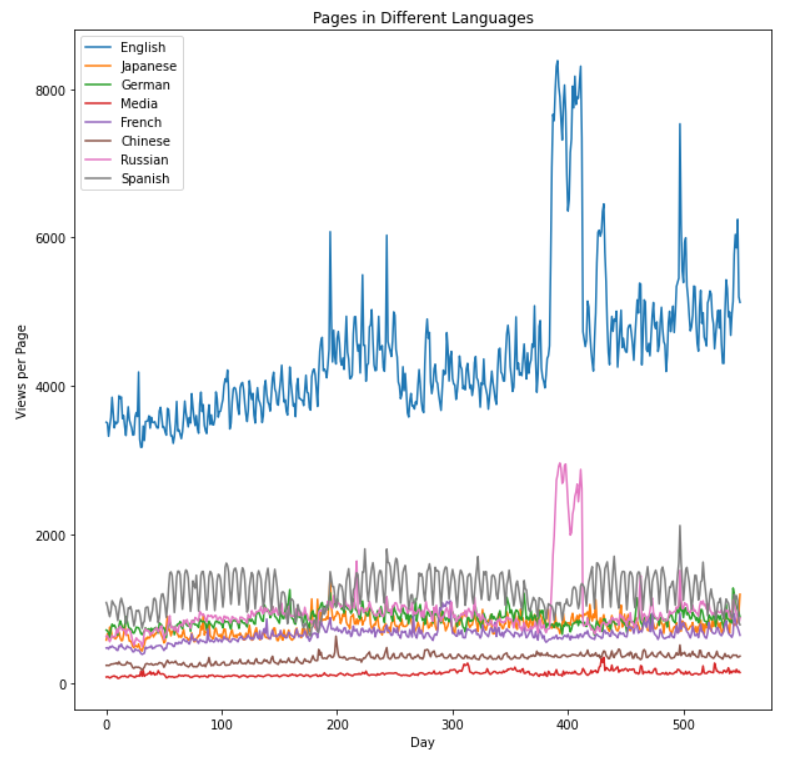
days = [r for r in range(sums['en'].shape[0])]

fig = plt.figure(1,figsize=[10,10])
plt.ylabel('Views per Page')
plt.xlabel('Day')
plt.title('Pages in Different Languages')
labels={'en':'English','ja':'Japanese','de':'German',
        'na':'Media','fr':'French','zh':'Chinese',
        'ru':'Russian','es':'Spanish'
       }

for key in sums:
    plt.plot(days,sums[key],label = labels[key] )

plt.legend()
plt.show()
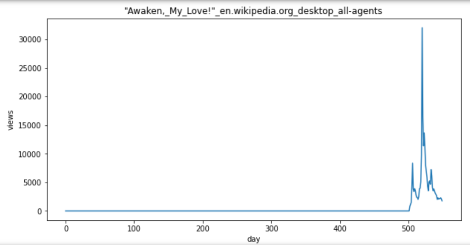
def plot_entry(key,idx):
    data = lang_sets[key].iloc[idx,1:]
    fig = plt.figure(1,figsize=(10,5))
    plt.plot(days,data)
    plt.xlabel('day')
    plt.ylabel('views')
    plt.title(train.iloc[lang_sets[key].index[idx],0])

    plt.show()
idx = [1, 5, 10, 50, 100, 250,500, 750,1000,1500,2000,3000,4000,5000]
for i in idx:
    plot_entry('en',i)
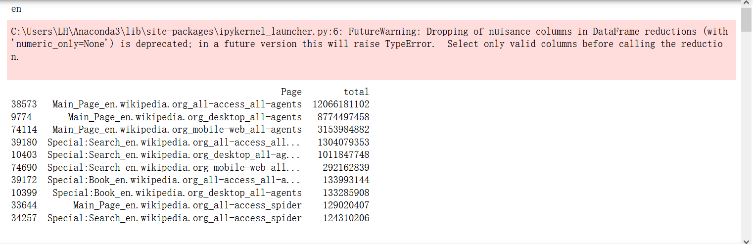
npages = 5
top_pages = {}
for key in lang_sets:
    print(key)
    sum_set = pd.DataFrame(lang_sets[key][['Page']])
    sum_set['total'] = lang_sets[key].sum(axis=1)
    sum_set = sum_set.sort_values('total',ascending=False)
    print(sum_set.head(10))
    top_pages[key] = sum_set.index[0]
    print('\n\n')
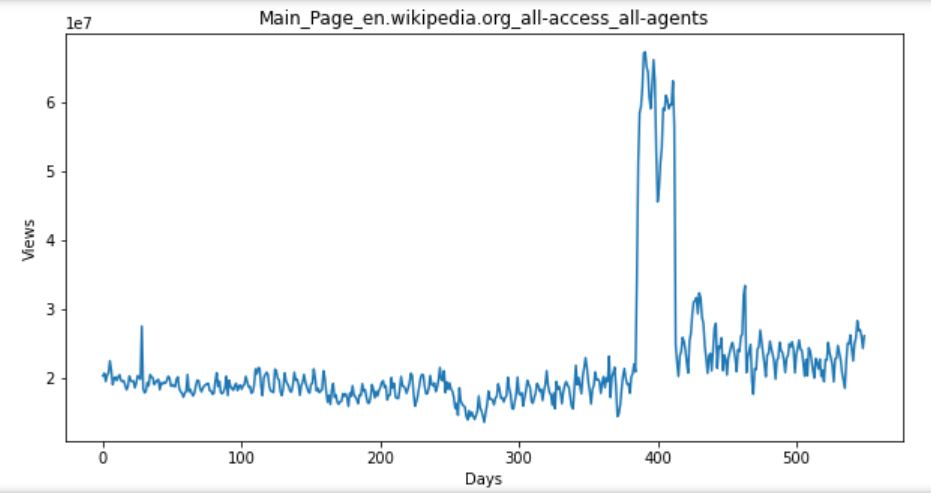
for key in top_pages:
    fig = plt.figure(1,figsize=(10,5))
    cols = train.columns
    cols = cols[1:-1]
    data = train.loc[top_pages[key],cols]
    plt.plot(days,data)
    plt.xlabel('Days')
    plt.ylabel('Views')
    plt.title(train.loc[top_pages[key],'Page'])
    plt.show()
Solutions to problems encountered
-
for train_k, test_k in KFold(len(train_kobe), n_folds=10, shuffle=True): many errors will be reported
Need to be changed to for train_k, test_k in KFold(10, shuffle=True).split(train_kobe): -
NameError: name 'dt' is not defined
Package not imported: import datetime as dt -
AttributeError: 'DataFrame' object has no attribute 'as_matrix'
Set corr = x.corr() as_ Matrix() [0] [1] changed to corr = x.corr() iloc[:,:]. values[0][1] -
ModuleNotFoundError: No module named 'pandas_datareader'
Generally, PIP install pandas is not installed_ datareader
-
model = ARIMA(stock_train, order=(1, 1, 1),freq = 'W-MON') reports an error notimplementederror: statsmodes tsa. arima_ model. ARMA and statsmodels. tsa. arima_ model. ARIMA have been removed in favor of statsmodels. tsa. arima. model. ARIMA (note the . between arima and model) and statsmodels. tsa. SARIMAX.
This is due to the abandonment of ARIMA package "statsmodes \ TSA \ arima_model".
So put this from stats models tsa. arima_ Model import Arima annotation, changed to import statsmodes API as SM, changed to model = SM when referenced tsa. arima. ARIMA(stock_train, order=(1, 1, 1),freq=‘W-MON’)
reference resources: https://stackoverflow.com/questions/67601211/futurewarning-statsmodels-tsa-arima-model-arma-and-statsmodels-tsa-arima-model -
download_robot_execution_failures() reported an error ConnectionError:
open https://github.com/MaxBenChrist/robot-failure-dataset/blob/master/lp1.data.txt , in https://github.com/MaxBenChrist/robot-failure-dataset Download code manually and Lp1 data. Txt manually copy to ~ / anaconda3 / lib / python3 8 / site packages / tsfresh / examples / data / robot failure MLD and renamed Lp1 data.
Reference articles https://blog.csdn.net/The_Time_Runner/article/details/110248835