SARIMA(p,d,q)(P,D,Q,s) seasonal autoregressive moving average model has seven structural parameters
AR(p) autoregressive model, i.e. use oneself to regress oneself.
The basic assumption is that the current sequence value depends on its previous value with time delay. The maximum lag in the model is recorded as p
To determine the initial p, you need to look at the PACF graph and find the largest significant lag, after which most of the other lags become irrelevant.
MA(q) moving average model is to model the error of time series, and assume that the current error depends on the error with delay. The initial value can be found on the ACF graph.
Combining the above two methods: AR(p)+MA(q)=ARMA(p,q)AR(p)+MA(q)=ARMA(p,q)AR(p)+MA(q)=ARMA(p,q), which is the autoregressive moving average model
Remaining parameters:
I(d)
- order of integration. This is simply the number of nonseasonal differences needed to make the series stationary. In our case, it's just 1 because we used first differences.
Adding this letter to the four gives us the ARIMA
model which can handle non-stationary data with the help of nonseasonal differences. Great, one more letter to go!
S(s)
- this is responsible for seasonality and equals the season period length of the series
With this, we have three parameters: (P,D,Q)
P
- order of autoregression for the seasonal component of the model, which can be derived from PACF. But you need to look at the number of significant lags, which are the multiples of the season period length. For example, if the period equals 24 and we see the 24-th and 48-th lags are significant in the PACF, that means the initial P
should be 2.
Q
- similar logic using the ACF plot instead.
D
- order of seasonal integration. This can be equal to 1 or 0, depending on whether seasonal differeces were applied or not.
OK, let's use SARIMA to model A kind of
Import package
import warnings                                  # do not disturbe mode
warnings.filterwarnings('ignore')

# Load packages
import numpy as np                               # vectors and matrices
import pandas as pd                              # tables and data manipulations
import matplotlib.pyplot as plt                  # plots
import seaborn as sns                            # more plots

from dateutil.relativedelta import relativedelta # working with dates with style
from scipy.optimize import minimize              # for function minimization

import statsmodels.formula.api as smf            # statistics and econometrics
import statsmodels.tsa.api as smt
import statsmodels.api as sm
import scipy.stats as scs

from itertools import product                    # some useful functions
from tqdm import tqdm_notebook

# Importing everything from forecasting quality metrics
from sklearn.metrics import r2_score, median_absolute_error, mean_absolute_error
from sklearn.metrics import median_absolute_error, mean_squared_error, mean_squared_log_error
# MAPE
def mean_absolute_percentage_error(y_true, y_pred):
    return np.mean(np.abs((y_true - y_pred) / y_true)) * 100

def tsplot(y, lags=None, figsize=(12, 7), style='bmh'):
    """
        Plot time series, its ACF and PACF, calculate Dickey–Fuller test

        y - timeseries
        lags - how many lags to include in ACF, PACF calculation
    """

    if not isinstance(y, pd.Series):
        y = pd.Series(y)

    with plt.style.context(style):
        fig = plt.figure(figsize=figsize)
        layout = (2, 2)
        ts_ax = plt.subplot2grid(layout, (0, 0), colspan=2)
        acf_ax = plt.subplot2grid(layout, (1, 0))
        pacf_ax = plt.subplot2grid(layout, (1, 1))

        y.plot(ax=ts_ax)
        p_value = sm.tsa.stattools.adfuller(y)[1]
        ts_ax.set_title('Time Series Analysis Plots\n Dickey-Fuller: p={0:.5f}'.format(p_value))
        smt.graphics.plot_acf(y, lags=lags, ax=acf_ax)
        smt.graphics.plot_pacf(y, lags=lags, ax=pacf_ax)
        plt.tight_layout()
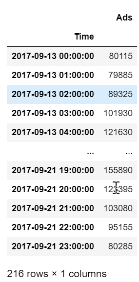
Read data
ads = pd.read_csv('ads.csv', index_col=['Time'], parse_dates=['Time'])
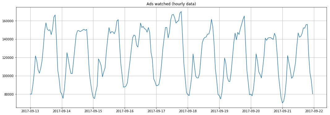
plt.figure(figsize=(18, 6))
plt.plot(ads.Ads)
plt.title('Ads watched (hourly data)')
plt.grid(True)
plt.show()
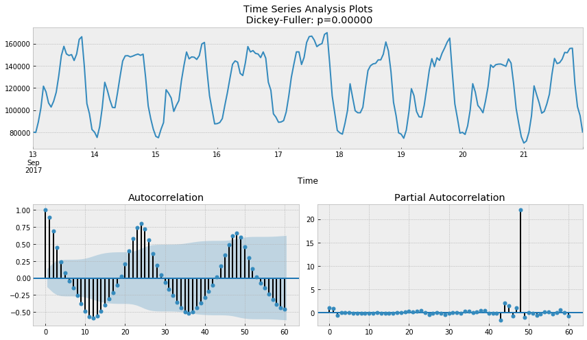
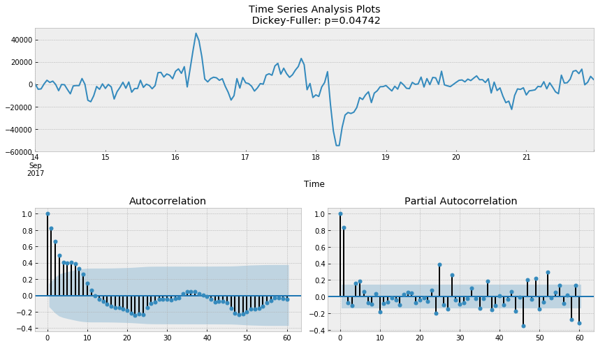
tsplot(ads.Ads, lags=60)
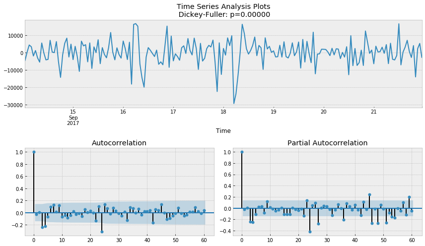
# The seasonal difference
ads_diff = ads.Ads - ads.Ads.shift(24)
tsplot(ads_diff[24:], lags=60)
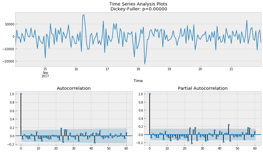
ads_diff = ads_diff - ads_diff.shift(1)
tsplot(ads_diff[24+1:], lags=60)
SARIMA parameter
- p is 4 because the last significant lag on the PACF, after which most of the others were not significant.
- d is 1 because of the first order difference
- q according to ACF, it should be about 4
- P may be 2, because the lag of 24 and 48 is important in PACF
- D is 1 because we do the seasonal difference
- Q may be 1, the 24th lag of ACF is obvious, while the 48th lag is not
# setting initial values and some bounds for them
ps = range(2, 5)
d=1
qs = range(2, 5)
Ps = range(0, 2)
D=1
Qs = range(0, 2)
s = 24 # season length is still 24

# creating list with all the possible combinations of parameters
parameters = product(ps, qs, Ps, Qs)
parameters_list = list(parameters)
len(parameters_list)  # 36
Adjust parameters according to AIC
def optimizeSARIMA(parameters_list, d, D, s):
    """Return dataframe with parameters and corresponding AIC

        parameters_list - list with (p, q, P, Q) tuples
        d - integration order in ARIMA model
        D - seasonal integration order
        s - length of season
    """

    results = []
    best_aic = float("inf")

    for param in tqdm_notebook(parameters_list):
        # we need try-except because on some combinations model fails to converge
        try:
            model=sm.tsa.statespace.SARIMAX(ads.Ads, order=(param[0], d, param[1]),
                                            seasonal_order=(param[2], D, param[3], s)).fit(disp=-1)
        except:
            continue
        aic = model.aic
        # saving best model, AIC and parameters
        if aic < best_aic:
            best_model = model
            best_aic = aic
            best_param = param
        results.append([param, model.aic])

    result_table = pd.DataFrame(results)
    result_table.columns = ['parameters', 'aic']
    # sorting in ascending order, the lower AIC is - the better
    result_table = result_table.sort_values(by='aic', ascending=True).reset_index(drop=True)

    return result_table
warnings.filterwarnings("ignore")
result_table = optimizeSARIMA(parameters_list, d, D, s)
'''
	 parameters	    aic
0	(2, 3, 1, 1)	3888.642174
1	(3, 2, 1, 1)	3888.763568
2	(4, 2, 1, 1)	3890.279740
3	(3, 3, 1, 1)	3890.513196
4	(2, 4, 1, 1)	3892.302849
5	(4, 3, 1, 1)	3892.322855
6	(3, 4, 1, 1)	3893.762846
7	(4, 4, 1, 1)	3894.327967
8	(2, 2, 1, 1)	3894.798147
9	(2, 3, 0, 1)	3897.170902
10	(3, 2, 0, 1)	3897.815032
11	(4, 2, 0, 1)	3899.073591
12	(3, 3, 0, 1)	3899.165271
13	(3, 4, 0, 1)	3900.500309
14	(2, 4, 0, 1)	3900.502494
15	(4, 3, 0, 1)	3901.255700
16	(4, 4, 0, 1)	3902.650501
17	(2, 2, 0, 1)	3903.905714
18	(2, 3, 1, 0)	3909.281188
19	(3, 2, 1, 0)	3909.502838
20	(4, 2, 1, 0)	3910.927759
21	(3, 3, 1, 0)	3911.192654
22	(3, 4, 1, 0)	3911.344351
23	(2, 4, 1, 0)	3911.809710
24	(4, 4, 1, 0)	3913.084053
25	(4, 3, 1, 0)	3913.409057
26	(2, 2, 1, 0)	3914.786853
27	(3, 2, 0, 0)	3925.433806
28	(2, 2, 0, 0)	3925.786566
29	(2, 3, 0, 0)	3925.879649
30	(2, 4, 0, 0)	3926.311190
31	(3, 3, 0, 0)	3927.427240
32	(4, 2, 0, 0)	3927.427417
33	(3, 4, 0, 0)	3928.376406
34	(4, 3, 0, 0)	3929.059361
35	(4, 4, 0, 0)	3930.078725
'''
# set the parameters that give the lowest AIC
p, q, P, Q = result_table.parameters[0]

best_model=sm.tsa.statespace.SARIMAX(ads.Ads, order=(p, d, q),
                                        seasonal_order=(P, D, Q, s)).fit(disp=-1)
print(best_model.summary())
'''
                                 Statespace Model Results
==========================================================================================
Dep. Variable:                                Ads   No. Observations:                  216
Model:             SARIMAX(2, 1, 3)x(1, 1, 1, 24)   Log Likelihood               -1936.321
Date:                            Sat, 07 Mar 2020   AIC                           3888.642
Time:                                    15:00:14   BIC                           3914.660
Sample:                                09-13-2017   HQIC                          3899.181
                                     - 09-21-2017
Covariance Type:                              opg
==============================================================================
                 coef    std err          z      P>|z|      [0.025      0.975]
------------------------------------------------------------------------------
ar.L1          0.7913      0.270      2.928      0.003       0.262       1.321
ar.L2         -0.5503      0.306     -1.799      0.072      -1.150       0.049
ma.L1         -0.7316      0.262     -2.793      0.005      -1.245      -0.218
ma.L2          0.5651      0.282      2.005      0.045       0.013       1.118
ma.L3         -0.1811      0.092     -1.964      0.049      -0.362      -0.000
ar.S.L24       0.3312      0.076      4.351      0.000       0.182       0.480
ma.S.L24      -0.7635      0.104     -7.361      0.000      -0.967      -0.560
sigma2      4.574e+07   5.61e-09   8.15e+15      0.000    4.57e+07    4.57e+07
===================================================================================
Ljung-Box (Q):                       43.70   Jarque-Bera (JB):                10.56
Prob(Q):                              0.32   Prob(JB):                         0.01
Heteroskedasticity (H):               0.65   Skew:                            -0.28
Prob(H) (two-sided):                  0.09   Kurtosis:                         4.00
===================================================================================

Warnings:
[1] Covariance matrix calculated using the outer product of gradients (complex-step).
[2] Covariance matrix is singular or near-singular, with condition number 1.08e+32. Standard errors may be unstable.
'''
tsplot(best_model.resid[24+1:], lags=60)
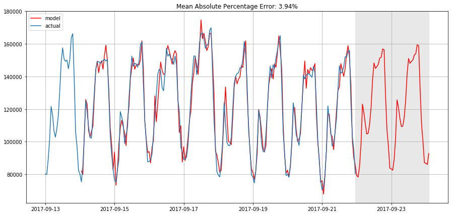
def plotSARIMA(series, model, n_steps):
    """Plots model vs predicted values

        series - dataset with timeseries
        model - fitted SARIMA model
        n_steps - number of steps to predict in the future
    """

    # adding model values
    data = series.copy()
    data.columns = ['actual']
    data['sarima_model'] = model.fittedvalues
    # making a shift on s+d steps, because these values were unobserved by the model
    # due to the differentiating
    data['sarima_model'][:s+d] = np.NaN

    # forecasting on n_steps forward
    forecast = model.predict(start = data.shape[0], end = data.shape[0]+n_steps)
    forecast = data.sarima_model.append(forecast)
    # calculate error, again having shifted on s+d steps from the beginning
    error = mean_absolute_percentage_error(data['actual'][s+d:], data['sarima_model'][s+d:])

    plt.figure(figsize=(15, 7))
    plt.title("Mean Absolute Percentage Error: {0:.2f}%".format(error))
    plt.plot(forecast, color='r', label="model")
    plt.axvspan(data.index[-1], forecast.index[-1], alpha=0.5, color='lightgrey')
    plt.plot(data.actual, label="actual")
    plt.legend()
    plt.grid(True)
plotSARIMA(ads, best_model, 50)