Blog Park address: https://www.cnblogs.com/LXP-Never/p/10078200.html

1. Introduction

python already supports writing in WAV format, but real-time sound input and output needs to be installed pyAudio . Finally, we'll use pyMedia Decode and play Mp3.

Audio signals are analog signals and need to be saved as digital signals to perform algorithm operations on speech. WAV is a sound file format developed by Microsoft and is often used to store uncompressed sound data.

Voice signal has four important parameters: number of channels, sampling frequency, quantization bits (bit depth) and bit rate.
Channel Number: Can be mono, dual channel...

• Sample rate: The total number of sound signal samples sampled per second at 44100Hz means that the signal is decomposed into 44100 copies per second. In other words, it is stored every 1/144100 seconds. If the sampling rate is high, the media will feel the signal is continuous when playing audio.
• Bit depth: Also known as bit depth, the number of bits of information in each sample point. 1 byte equals 8 bit s. Usually 8bit, 16bit, 24bit, 32bit...
• Bit rate: How many Bit s are processed per second. For example, for a mono channel, with a 44.1KHz/16Bit configuration, its bit rate is 441,00161=705600, in bit s/s (or bps), because the calculated number is usually large, so everyone uses kbit/s, or 705.6kbit/s. When compressing audio, bit rate becomes one of our choices. The higher the bit rate, the better the sound quality. Some commonly used bit rates are:

       - 32kbit/s:  Generally only for voice
       - 96kbit/s:  Commonly used for voice or low quality streaming
	   - 128 Or 160 kbit/s:  Medium bit rate quality
	   -  192kbit/s:  Medium quality bit rate
	   -  256kbit/s:  Commonly used high quality bit rates
	   -  320kbit/s:  MP3 The highest level of standard support

If you need to record and edit sound files yourself, Audacity, an open source, cross-platform, multi-channel recording editing software, is recommended. Audacity is often used in my work to record sound signals and then output them to WAV files for Python processing.
3
If you want a quick look at the voice waveforms and spectrograms, Adobe Audition is recommended. Adobe develops professional software for audio processing. Weibo pays attention to vposy and the download address is at the top. He cracked a lot of adobe's software, including PS, PR...

2. Read audio files

• wave Library

The wave library is the standard library for python. For python, wave does not support compression/decompression, but supports reading mono/stereo speech.

wave_read = wave.open(file,mode="rb")

Parameters:

f: Voice file name or file path
mode: Read or write
"rb": read only mode
"wb": Write-only mode
 Return: Read stream

The open() function can be used in the with declaration. When the with block is complete, wave_read.close() or wave_write.close() method called

File path:
For example, voice. The wav file is in the folder at path C:\Users\Never\Desktop\code for the speech
file has three filling formats:
　　　　r"C:\Users\Never\Desktop\code for the speech\voice.wav"
　　　　"C:/Users/Never/Desktop/code for the speech/voice.wav"
　　　　"C:\Users\Never\Desktop\code for the speech\voice.wav"
The three are equivalent, the right dash \ is an ideographic character, and \ is required if \ is to be expressed, and the quotation mark preceded by r denotes the original string.

wave_read.getparams(): Returns all the audio parameters at once, returning a tuple (number of channels, number of quantifiable bits (byte units), sampling frequency, number of samples, compression type, description of compression type). (nchannels, sampwidth, framerate, nframes, comptype, compname)wave module only supports uncompressed data, so the last two information can be ignored.

str_data = wave_read.readframes(nframes): The length of the read (in sampling points) that returns data of type string

wave_data = np.fromstring(str_data, dtype=np.float16): Converts the above string type data to an array of one-dimensional float16 types.

Now wave_data is a one-dimensional short-type array, but because our sound file is two-channel, it consists of two alternating channels: LR

wave_data.shape = (-1, 2) # -1 means unspecified, divided by the number of other dimensions to get an array of n rows and 2 columns.

wave_read.close()　　Close File Stream wave
wave_read.getnchannels()　　Returns the number of audio channels (1 for mono and 2 for stereo).
wave_read.getsampwidth()　　Returns the sample width in bytes
wave_read.getframerate()　　Returns the sampling frequency.
wave_read.getnframes()　　　Returns the number of audio frames.
wave_read.rewind()　　　　　　Reverse the file pointer back to the beginning of the audio stream.
wave_read.tell()　　　　　　Returns the current file pointer position. 

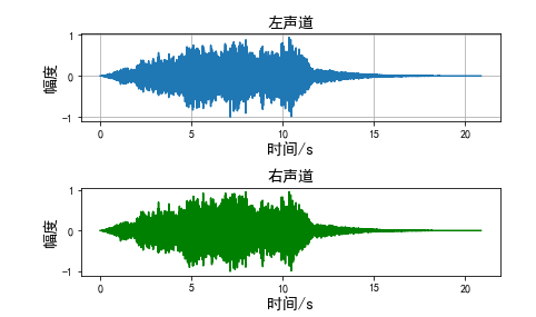
Read the Wave file and draw the waveform

# -*- coding: utf-8 -*-
# Read the Wave file and draw the waveform
import wave
import matplotlib.pyplot as plt
import numpy as np

plt.rcParams['font.sans-serif'] = ['SimHei']  # Used for normal display of Chinese labels
plt.rcParams['axes.unicode_minus'] = False  # Used to display symbols normally

# Turn on WAV audio
f = wave.open(r"C:\Windows\media\Windows Background.wav", "rb")

# Read format information
# (description of channel number, quantization number, sampling frequency, sampling number, compression type, compression type)
# (nchannels, sampwidth, framerate, nframes, comptype, compname)
params = f.getparams()
nchannels, sampwidth, framerate, nframes = params[:4]
# Number of nchannels channels = 2
# sampwidth quantifier = 2
# Frameerate sampling frequency = 22050
# nframes sample number = 53395

# Read nframes data, return string format
str_data = f.readframes(nframes)

f.close()

# Converts a string to an array to get an array of one-dimensional short type
wave_data = np.fromstring(str_data, dtype=np.short)

# Normalization of assignments
wave_data = wave_data * 1.0 / (max(abs(wave_data)))

# Integrating data from left and right channels
wave_data = np.reshape(wave_data, [nframes, nchannels])
# wave_data.shape = (-1, 2)   # The meaning of -1 is that it is unspecified, divided by the number of other dimensions

# Finally, each sampling time is calculated from the number of points sampled and the sampling frequency.
time = np.arange(0, nframes) * (1.0 / framerate)

plt.figure()
# Left Channel Waveform
plt.subplot(2, 1, 1)
plt.plot(time, wave_data[:, 0])
plt.xlabel("time/s",fontsize=14)
plt.ylabel("Range",fontsize=14)
plt.title("Left channel",fontsize=14)
plt.grid()  # Ruler

plt.subplot(2, 1, 2)
# Right Channel Waveform
plt.plot(time, wave_data[:, 1], c="g")
plt.xlabel("time/s",fontsize=14)
plt.ylabel("Range",fontsize=14)
plt.title("Right",fontsize=14)

plt.tight_layout()  # Tight Layout
plt.show()

Read audio signal with 2 channels

If an error occurs: np.fromstring string size must be a multiple of element size
Reference solutions: https://blog.csdn.net/veritasalice/article/details/104807415

• librosa library (recommended)

This is my most commonly used and favorite voice library. Librosa is a third-party python library. Before using it, we need to run on a cmd terminal: pip install librosa. I wrote a blog about librosa voice signal processing specifically.

import librosa
y, sr = librosa.load(path, sr=fs)

This function changes the sampling frequency of sound. If sr is default, librosa.load() reads audio files at a sampling rate of 22050 by default. Audio files above this sampling rate are downsampled and files below this sampling rate are uploaded. Therefore, if you want to read the audio file at the original sampling rate, sr should be set to None. This is y, sr = librosa(filename, sr=None).
Audio data y is a directly normalized array

• scipy Library

from scipy.io import wavfile
sampling_freq, audio = wavfile.read("***.wav")

audio is a directly normalized array

3. Write audio files

• wave Library

When writing the first frame data, set the number of frames by calling setnframes(), set nchannels (), set sampwidth (), set the quantization bits, set framerate () set the sampling frequency, and then writeframes(wave.tostring()) are used to write the frame data.

wave_write = wave.open(file,mode="wb") 

wave_write is a write file stream

wave_write.setnchannels(n)　　Set the number of channels.
wave_write.setsampwidth(n)　　Set sample width to n Bytes, quantized bits
wave_write.setframerate(n)　　Set sampling frequency to n. 
wave_write.setnframes(n)　　Set the number of frames to n
wave_write.setparams(tuple)　　Set all parameters as tuples(nchannels, sampwidth, framerate, nframes,comptype, compname)
wave_write.writeframes(data)　　Write in data Audio of length, in sampling points
wave_write.tell()　　Returns the current position in the file

• Write wav file
  Write File Method 1

# Author:Ling Ren Battle
# -*- coding:utf-8 -*-
import wave
import numpy as np
import scipy.signal as signal

framerate = 44100   # sampling frequency
time = 10           # Duration

t = np.arange(0, time, 1.0/framerate)

# Call scipy. The chrip function in the signal library,
# Frequency scan waves with length of 10 seconds, sampling frequency of 44.1 kHz, 100Hz to 1kHz are generated
wave_data = signal.chirp(t, 100, time, 1000, method='linear') * 10000

# Because the array returned by the chrip function is float64,
# The astype method of the array needs to be invoked to convert it to short.
wave_data = wave_data.astype(np.short)

# Turn on WAV audio for write operations
f = wave.open(r"sweep.wav", "wb")

f.setnchannels(1)           # Configure Channel Number
f.setsampwidth(2)           # Configure Quantity Bits
f.setframerate(framerate)   # Configure sampling frequency
comptype = "NONE"
compname = "not compressed"

# You can also configure all parameters at once with setparams
# outwave.setparams((1, 2, framerate, nframes,comptype, compname))

# Will wav_data converted to binary data write file
f.writeframes(wave_data.tobytes())
f.close()

Write WAV File Method 2

# Author:Ling Ren Battle
# -*- coding:utf-8 -*-
import wave
import numpy as np
import struct

f = wave.open(r"C:\Windows\media\Windows Background.wav", "rb")
params = f.getparams()
nchannels, sampwidth, framerate, nframes = params[:4]
strData = f.readframes(nframes)
waveData = np.fromstring(strData,dtype=np.int16)
f.close()
waveData = waveData*1.0/(max(abs(waveData)))

# wav file write
# Data to be written to wav, waveData data is still fetched here
outData = waveData
outwave = wave.open("write.wav", 'wb')
nchannels = 1   # Number of channels set to 1
sampwidth = 2   # Quantitative Bit Set to 2
framerate = 8000    # Sampling frequency 8000
nframes = len(outData)    # Sample Points

comptype = "NONE"
compname = "not compressed"
outwave.setparams((nchannels, sampwidth, framerate, nframes,
    comptype, compname))

for i in outData:
        outwave.writeframes(struct.pack('h', int(i * 64000 / 2)))

        # struct.pack(FMT, V1) converts the value of V1 to an FMT format string
outwave.close()

• librosa library (recommended)

librosa.output.write_wav(path, y, sr, norm=False)

Parameters:

path: str，Save Output wav Path to file
y: np.ndarry Audio Time Series
sr: y Sampling rate of
norm: True/False，Whether to start amplitude normalization

At 0.8. In versions later than 0, librosa will delete this function. The following functions are recommended:

import soundfile
soundfile.write(file, data, samplerate)

Parameters:

file: Save Output wav Path to file
data: Audio data
samplerate: sampling rate

• scipy Library

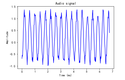
from scipy.io.wavfile import write
write(output_filename, freq, audio)

import numpy as np
import matplotlib.pyplot as plt
from scipy.io.wavfile import write

# Define output file to store audio
output_file = 'output_generated.wav'

# Specify parameters for audio generation
duration = 3            # Unit seconds
sampling_freq = 44100   # Unit Hz
tone_freq = 587         # Frequency of tones
min_val = -2 * np.pi
max_val = 2 * np.pi

# Generate audio signal
t = np.linspace(min_val, max_val, duration * sampling_freq)
audio = np.sin(2 * np.pi * tone_freq * t)

# Adding noise (random values between duration * sampling_freq (0,1))
noise = 0.4 * np.random.rand(duration * sampling_freq)
audio += noise

scaling_factor = pow(2,15) - 1  # Convert to 16-bit integer
audio_normalized = audio / np.max(np.abs(audio))    # normalization
audio_scaled = np.int16(audio_normalized * scaling_factor)  # What does this sentence mean?

write(output_file, sampling_freq, audio_scaled) # Write Output File

audio = audio[:300] # Get the first 300 audio signals

x_values = np.arange(0, len(audio), 1) / float(sampling_freq)
x_values *= 1000    # Convert timeline units to seconds

plt.plot(x_values, audio, color='blue')
plt.xlabel('Time (ms)')
plt.ylabel('Amplitude')
plt.title('Audio signal')
plt.show()

• Synthesize tuned music

import json
import numpy as np
from scipy.io.wavfile import write
import matplotlib.pyplot as plt          

# Define composite tones
def Synthetic_tone(freq, duration, amp=1.0, sampling_freq=44100):
    # Establish timeline
    t = np.linspace(0, duration, int(duration * sampling_freq))
    # Build audio signal
    audio = amp * np.sin(2 * np.pi * freq * t)
    return audio.astype(np.int16)


# The json file contains some scales and their frequencies
tone_map_file = 'tone_freq_map.json'

# Read Frequency Mapping File
with open(tone_map_file, 'r',encoding='UTF-8') as f:
    tone_freq_map = json.loads(f.read())
    print(tone_freq_map)
# {'A': 440, 'Asharp': 466, 'B': 494, 'C': 523, 'Csharp': 554, 'D': 587, 'Dsharp': 622, 'E': 659, 'F': 698, 'Fsharp': 740, 'G': 784, 'Gsharp': 831}

# Set input parameters to generate G-tone
input_tone = 'G'
duration = 2             # seconds
amplitude = 10000        # amplitude
sampling_freq = 44100    # Hz
# Generate scale
synthesized_tone = Synthetic_tone(tone_freq_map[input_tone], duration, amplitude, sampling_freq)

# Write Output File
write('output_tone.wav', sampling_freq, synthesized_tone)

# Scale and its continuous time
tone_seq = [('D', 0.3), ('G', 0.6), ('C', 0.5), ('A', 0.3), ('Asharp', 0.7)]

# Building an Audio Signal Based on Chord Sequence
output = np.array([])
for item in tone_seq:
    input_tone = item[0]
    duration = item[1]
    synthesized_tone = Synthetic_tone(tone_freq_map[input_tone], duration, amplitude, sampling_freq)
    output = np.append(output, synthesized_tone, axis=0)

# Write Output File
write('output_tone_seq.wav', sampling_freq, output)

tone_freq_map.json

{
    "A": 440,
    "Asharp": 466,
    "B": 494,
    "C": 523,
    "Csharp": 554,
    "D": 587,
    "Dsharp": 622,
    "E": 659,
    "F": 698,
    "Fsharp": 740,
    "G": 784,
    "Gsharp": 831
}

-Audio playback
The pyaudio library is used for playing wav files
P = pyaudio. PyAudio() stream = p.open (format = p.get_format_from_width), channels, rate, output = True) stream. Write (data) #Play data data

The main parameters for the open() method of the pyaudio object are listed below:

rate: sampling frequency
Channels: number of channels
Format: Quantitative format of the sampled values (paFloat32, paInt32, paInt24, paInt16, paInt8...). In the example above, use get_ Format_ From_ The width method will wf. The return value of sampwidth() 2 is converted to paInt16
Input: Input stream flag, open input stream if True
Output: Output stream flag, turn on output stream if True
input_device_index: The number of the device used by the input stream, if not specified, the default device of the system is used
output_device_index: The number of the device used by the output stream, if not specified, the default device of the system is used
frames_per_buffer: The size of the underlying cache block, which consists of N blocks of the same size
start: Specifies whether the input and output streams will be opened immediately, with a default value of True

Play wav audio

# -*- coding: utf-8 -*-
import pyaudio
import wave

chunk = 1024
wf = wave.open(r"c:\WINDOWS\Media\Windows Background.wav", 'rb')
p = pyaudio.PyAudio()

# Turn on sound output stream
stream = p.open(format = p.get_format_from_width(wf.getsampwidth()),
                channels = wf.getnchannels(),
                rate = wf.getframerate(),
                output = True)

# Write sound output stream to sound card for playback
while True:
    data = wf.readframes(chunk)
    if data == "":
        break
    stream.write(data)

stream.stop_stream()
stream.close()
p.terminate()   # Close PyAudio

Sound recording

With SAMPLING_RATE is the sampling frequency, with NUM_in each read block SAMPLES Sampled Data Blocks, when COUNT_is in the read sample data When NUM values are larger than LEVEL samples, save the data into a WAV file, once the data is saved, the minimum length of the data saved is SAVE_LENGTH blocks. The WAV file is named the moment it was saved.

The data read from the sound card is binary, similar to the data read from the WAV file. Since we save the sample values in paInt16 format (short type of 16bit), we convert it to dtype to np. Array of shorts.

'''
with SAMPLING_RATE For sampling frequency,
Read one block at a time with NUM_SAMPLES Data blocks of sample points,
When the sample data read in has COUNT_NUM Values greater than LEVEL When sampling,
Save Sampled Data in WAV Files,
Once you start saving your data, you can save it as short as SAVE_LENGTH Data blocks.

Data read from sound card and from WAV Files read like binary data.
Because we use paInt16 format(16bit Of short type)Save the sample values,
So convert itself to dtype by np.short Array.
'''


from pyaudio import PyAudio, paInt16
import numpy as np
import wave

# Save the data in the data to a WAV file named filename
def save_wave_file(filename, data):
    wf = wave.open(filename, 'wb')
    wf.setnchannels(1)          # single channel
    wf.setsampwidth(2)          # Quantization Bits
    wf.setframerate(SAMPLING_RATE)  # Set Sampling Frequency
    wf.writeframes(b"".join(data))  # Write Voice Frame
    wf.close()


NUM_SAMPLES = 2000      # Size of pyAudio internal cache block
SAMPLING_RATE = 8000    # Sampling frequency
LEVEL = 1500           # The threshold for sound preservation, below which no recording occurs
COUNT_NUM = 20 # Cached Fast Class Records sound if there are 20 samples larger than the threshold
SAVE_LENGTH = 8 # Minimum length of sound recording: SAVE_LENGTH * NUM_SAMPLES Samples

# Turn on sound input
pa = PyAudio()
stream = pa.open(format=paInt16, channels=1, rate=SAMPLING_RATE, input=True,
                frames_per_buffer=NUM_SAMPLES)

save_count = 0  # To count
save_buffer = []    #

while True:
    # Read in NUM_SAMPLES Samples
    string_audio_data = stream.read(NUM_SAMPLES)
    # Convert read data to an array
    audio_data = np.fromstring(string_audio_data, dtype=np.short)
    # Calculate the number of samples larger than LEVEL
    large_sample_count = np.sum( audio_data > LEVEL )
    print(np.max(audio_data))
    # If the number is greater than COUNT_NUM, then save at least SAVE_LENGTH Blocks
    if large_sample_count > COUNT_NUM:
        save_count = SAVE_LENGTH
    else:
        save_count -= 1

    if save_count < 0:
        save_count = 0

    if save_count > 0:
        # Store the data to be saved in save_ In buffer
        save_buffer.append( string_audio_data )
    else:
        # Will save_ The data in the buffer is written to the WAV file whose filename is the time of saving
        if len(save_buffer) > 0:
            filename = "recorde" + ".wav"
            save_wave_file(filename, save_buffer)
            print(filename, "saved")
            break

3. Speech signal processing

3.1 Generation and perception of voice signal

To analyze speech, we must first extract the characteristic parameters that can represent the speech. Only with these parameters can we use them for effective processing. In the process of processing voice signal, the quality of voice signal depends not only on the processing method, but also on the selection of appropriate feature parameters.

Voice signal is a non-stationary time-varying signal, but voice signal is formed by the stimulation pulse of the glottis through the vocal channel, and the muscle movement of the vocal channel (human mouth, nose) is slow, so the voice signal can be considered stationary and unchanged in a "short time" (10-30ms). This constitutes the "short-time analysis technique" of voice signal.

In short-term analysis, voice signal is divided into a segment of voice frames, each frame is usually 10-30 Ms. Our research is based on the analysis of the voice characteristics of each frame.

Different speech feature parameters extracted correspond to different voice signal analysis methods: time domain analysis, frequency domain analysis, cepstrum domain analysis... Since the most important perception characteristics of voice signal are reflected in the power spectrum, and phase change plays a small role, all speech frequency domain analysis is more important.

3.2 Signal windowing

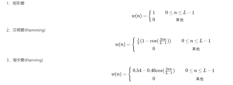
Generally, window is needed for signal truncation and framing, because truncation always leaks energy in frequency domain, and window function can reduce the impact of truncation.
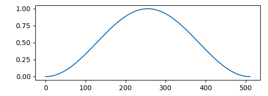
Window function in scipy. In the signal signal signal processing toolbox, such as the hanning window:

import matplotlib.pyplot as plt
import scipy.signal as signal
plt.figure(figsize=(6,2))
plt.plot(signal.hanning(512))
plt.show()

3.3 signal framing

In framing, there will be some overlap between adjacent frames, the frame length ( w l e n wlen wlen) =overlap ( o v e r l a p overlap overlap) + frame shift ( i n c inc inc), if there is no overlap between adjacent frames, then due to the shape of the window function, the captured voice frame edge will be lost, so the overlap will be set. i n c inc inc is a frame shift, which represents the offset of the next frame from the previous frame. f s f_s fs is the sampling rate, f n f_n fn Represents the number of frames of a voice signal.

N − o v e r l a p i n c = N − w l e n + i n c i n c \frac{N-overlap}{inc}=\frac{N-wlen+inc}{inc} incN−overlap​=incN−wlen+inc​
The theoretical basis of signal framing, where x x x is the voice signal, w w w is a window function:
y ( n ) = ∑ − n = N 2 + 1 N 2 x ( m ) w ( n − m ) y(n)=\sum_{-n=\frac{N}{2}+1}^{\frac{N}{2}}x(m)w(n-m) y(n)=−n=2N​+1∑2N​​x(m)w(n−m)

Window truncation is similar to sampling. In order to ensure that adjacent frames do not differ too much, there is usually a frame shift between frames, which is actually the function of interpolation smoothing.

Give a diagram:

This is mainly used with the numpy toolkit, which covers the following instructions:

np.repeat: Mainly direct repetition
np.tile: Mainly cyclical

Compare:
Vector case:

Matrix case:
For data

repeat operation:

tile operation:

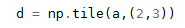
Corresponding results:

Code implementation for corresponding framing:
This is an example without windows:

• Voice framing without windowing

import numpy as np
import wave
import os
#import math

def enframe(signal, nw, inc):
   '''Converts an audio signal to a frame.
   Parameter meaning:
   signal:Original Audio Model
   nw:Length of each frame(This refers to the length of the sample point, that is, the sampling frequency multiplied by the time interval)
   inc:Interval between adjacent frames (as defined above)
   '''
   signal_length=len(signal) #Total Signal Length
   if signal_length<=nw: #If the signal length is less than the length of a frame, the number of frames is defined as 1
       nf=1
   else: #Otherwise, calculate the total length of the frame
       nf=int(np.ceil((1.0*signal_length-nw+inc)/inc))
   pad_length=int((nf-1)*inc+nw) #Total paved length of all frames combined
   zeros=np.zeros((pad_length-signal_length,)) #Insufficient length filled with 0, similar to expanded array operation in FFT
   pad_signal=np.concatenate((signal,zeros)) #The filled signal is marked as pad_signal
   indices=np.tile(np.arange(0,nw),(nf,1))+np.tile(np.arange(0,nf*inc,inc),(nw,1)).T  #Equivalent to extracting the time points of all frames to get a matrix of nf*nw lengths
   indices=np.array(indices,dtype=np.int32) #Converting indices to matrices
   frames=pad_signal[indices] #Get Frame Signal
#    win=np.tile(winfunc(nw),(nf,1))  #Window window function, default here is 1
#    return frames*win   #Return Frame Signal Matrix
   return frames
def wavread(filename):
   f = wave.open(filename,'rb')
   params = f.getparams()
   nchannels, sampwidth, framerate, nframes = params[:4]
   strData = f.readframes(nframes)#Read audio, string format
   waveData = np.fromstring(strData,dtype=np.int16)#Convert string to int
   f.close()
   waveData = waveData*1.0/(max(abs(waveData)))#wave amplitude normalization
   waveData = np.reshape(waveData,[nframes,nchannels]).T
   return waveData

filepath = "./data/" #Add Path
dirname= os.listdir(filepath) #Get all the file names under the folder 
filename = filepath+dirname[0]
data = wavread(filename)
nw = 512
inc = 128
Frame = enframe(data[0], nw, inc) 

• Windowed voice framing

def enframe(signal, nw, inc, winfunc):
    '''Converts an audio signal to a frame.
    Parameter meaning:
    signal:Original Audio Model
    nw:Length of each frame(This refers to the length of the sample point, that is, the sampling frequency multiplied by the time interval)
    inc:Interval between adjacent frames (as defined above)
    '''
    signal_length=len(signal) #Total Signal Length
    if signal_length<=nw: #If the signal length is less than the length of a frame, the number of frames is defined as 1
        nf=1
    else: #Otherwise, calculate the total length of the frame
        nf=int(np.ceil((1.0*signal_length-nw+inc)/inc))
    pad_length=int((nf-1)*inc+nw) #Total paved length of all frames combined
    zeros=np.zeros((pad_length-signal_length,)) #Insufficient length filled with 0, similar to expanded array operation in FFT
    pad_signal=np.concatenate((signal,zeros)) #The filled signal is marked as pad_signal
    indices=np.tile(np.arange(0,nw),(nf,1))+np.tile(np.arange(0,nf*inc,inc),(nw,1)).T  #Equivalent to extracting the time points of all frames to get a matrix of nf*nw lengths
    indices=np.array(indices,dtype=np.int32) #Converting indices to matrices
    frames=pad_signal[indices] #Get Frame Signal
    win=np.tile(winfunc,(nf,1))  #Window window function, default here is 1
    return frames*win   #Return Frame Signal Matrix

• overlap and add
  Split the framed speech back into the complete speech

def overlap_add(x, window_size, hop_size):
    # x (frames, frame_length)
    frames, frame_length = x.shape
    wav_len = frames * hop_size + window_size - hop_size  # Frame length
    print("Frame length", wav_len)
    wav = np.zeros((wav_len,), dtype=x.dtype)

    for frame in range(frames):
        if frame == frames - 1:
            # Last Frame
            wav[hop_size * frame: hop_size * frame + window_size] += x[frame]  # Add whole frame in front
        else:
            wav[hop_size * frame: hop_size * frame + hop_size] += x[frame][:hop_size]  # Add in front of frame

    return wav

3.4 Speech signal processing in short time domain

Short-time energy and short-time mean amplitude

Main uses of short-term energy and short-term mean amplitude:

• Distinguish between voiced and clear sounds because the short energy E(i)E(i) of voiced sounds is much higher than that of clear sounds.
• Distinguish between initial and vowel and between NO and segmental
  Short Time Average Cross zero ratio

For continuous voice signals, the zero-crossing rate means that the time-domain waveform passes through the time axis, and for discrete signals, if the adjacent sample values change the symbol, it is called zero-crossing.

Effect:

• Voiced voice signal energy is concentrated below 3kHz due to the high frequency drop of the spectrum caused by glottic wave.
• Most of the energy is focused on a higher frequency when the voice is articulated.

Because high frequencies mean high short average zero-crossing rates and low frequencies mean low short average zero-crossing rates, voiced sounds have lower zero-crossing rates and clear sounds have higher zero-crossing rates.

1.The short average zero-crossing rate can be used to find the voice signal from the background noise.
2.It can be used to determine the starting and ending positions of silent and silent segments.
3.Average energy is more effective when background noise is low, and short average zero-crossing rate is more effective when background noise is high.

Short-time autocorrelation function

Short-time autocorrelation functions are mainly used for endpoint detection and pitch extraction. Peak characteristics occur at integer times of the vowel gene frequency. The pitch is usually estimated based on the first peak except R(0), but no significant peak is seen in the short-time autocorrelation function of the initial.

Short-time mean amplitude difference function

It is used to detect pitch cycles and is more computationally simple than a short autocorrelation function.

Short-time frequency domain processing of voice signals
In speech signal processing, signal analysis and processing play an important role in frequency domain or other transform domain. Studying speech in frequency domain can make some features of the signal that can not be displayed in time domain obvious. The nature of an audio signal is determined by its frequency content.

Converting a time-domain signal to a frequency-domain signal generally performs a short-time Fourier transformation of the speech.

fft_audio = np.fft.fft(audio)

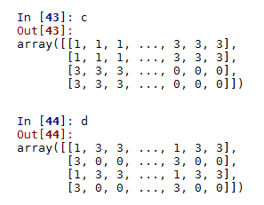
Draw the spectrum of voice signal

import numpy as np
from scipy.io import wavfile
import matplotlib.pyplot as plt

sampling_freq, audio = wavfile.read(r"C:\Windows\media\Windows Background.wav")   # read file

audio = audio / np.max(audio)   # Normalization, Standardization

# Applying Fourier Transform
fft_signal = np.fft.fft(audio)
print(fft_signal)
# [-0.04022912+0.j         -0.04068997-0.00052721j -0.03933007-0.00448355j
#  ... -0.03947908+0.00298096j -0.03933007+0.00448355j -0.04068997+0.00052721j]

fft_signal = abs(fft_signal)
print(fft_signal)
# [0.04022912 0.04069339 0.0395848  ... 0.08001755 0.09203427 0.12889393]

# Establish timeline
Freq = np.arange(0, len(fft_signal))

# Drawing voice signal
plt.figure()
plt.plot(Freq, fft_signal, color='blue')
plt.xlabel('Freq (in kHz)')
plt.ylabel('Amplitude')
plt.show()

• Extracting Frequency Domain Features
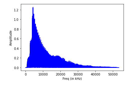
  After converting the signal into the frequency domain, it also needs to be converted into a useful form, Meyer Frequency Cepstrum Coefficient (MFCC), which first calculates the power spectrum of the signal, then extracts the characteristics using a combination of filter banks and discrete cosine transformations.

Extracting MFCC Features

import numpy as np
import matplotlib.pyplot as plt
from scipy.io import wavfile
from python_speech_features import mfcc, logfbank

# Read Input Audio File
sampling_freq, audio = wavfile.read("input_freq.wav")

# Extracting MFCC and filter bank characteristics
mfcc_features = mfcc(audio, sampling_freq)
filterbank_features = logfbank(audio, sampling_freq)

print('\nMFCC:\n Number of windows =', mfcc_features.shape[0])
print('Length of each feature =', mfcc_features.shape[1])
print('\nFilter bank:\n Number of windows =', filterbank_features.shape[0])
print('Length of each feature =', filterbank_features.shape[1])

# Draw a feature map to visualize MFCC. Transpose the matrix so that the time domain is horizontal
mfcc_features = mfcc_features.T
plt.matshow(mfcc_features)
plt.title('MFCC')
# Visualize filter bank characteristics. Transpose the matrix so that the time domain is horizontal
filterbank_features = filterbank_features.T
plt.matshow(filterbank_features)
plt.title('Filter bank')

plt.show()

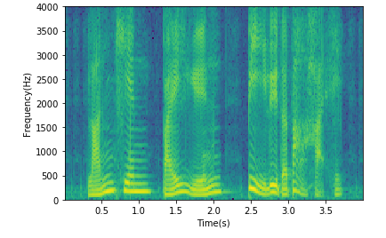
Spectrogram

Most signals can be decomposed into several sinusoidal waves of different frequencies.
Of these sinusoids, the lowest frequency is called the fundamental wave of the signal, and the rest are called the harmonics of the signal.
There is only one fundamental wave, which can be called first harmonic. There can be many harmonics, each harmonic frequency is an integer multiple of the fundamental frequency. Harmonics may vary in size.
A series of bar graphs drawn with the frequency of harmonics in the x-coordinate and the amplitude (size) in the p-coordinate are called the spectrum, which accurately reflects the internal structure of the signal.

Spectrogram combines the characteristics of time and frequency domains. It clearly shows the change of speech frequency over time. The horizontal axis of the spectrum is time, and the vertical axis is the intensity of any given frequency component at a given time. Color depth indicates a large spectrum value, light color indicates a small spectrum value, and different black and white levels on the spectrum form different patterns, called voice print. Without the speaker, voice print is different and can be used for voice print recognition.
In fact, we get the framing signal, frequency domain transformation to take the amplitude, you can get the spectrogram, if only observation, matplotlib.pyplot has specgram directives:

import wave
import matplotlib.pyplot as plt
import numpy as np

f = wave.open(r"C:\Windows\media\Windows Background.wav", "rb")
params = f.getparams()
nchannels, sampwidth, framerate, nframes = params[:4]
strData = f.readframes(nframes)#Read audio, string format
waveData = np.fromstring(strData,dtype=np.int16)#Convert string to int
waveData = waveData*1.0/(max(abs(waveData)))#wave amplitude normalization
waveData = np.reshape(waveData,[nframes,nchannels]).T
f.close()

plt.specgram(waveData[0],Fs = framerate, scale_by_freq = True, sides = 'default')
plt.ylabel('Frequency(Hz)')
plt.xlabel('Time(s)')
plt.show()

matlab Spectrogram

[Y,FS]=audioread('p225_355_wb.wav');

% specgram(Y,2048,44100,2048,1536);
    %Y1 For waveform data
    %FFT Frame length 2048 points(At 44100 Hz About 46 at frequency ms)
    %Sampling frequency 44.1KHz
    %Window length, generally equal to frame length
    %Frame overlap length, 3 of frame length here/4
specgram(Y,2048,FS,2048,1536);
xlabel('time(s)')
ylabel('frequency(Hz)')
title('Spectrogram')

3.5 Speech Recognition

import os
import numpy as np
import scipy.io.wavfile as wf
import python_speech_features as sf
import hmmlearn.hmm as hl


# 1. Read training audio samples in the training folder, one mfcc matrix for each audio, and one category for each mfcc (apple...)
def search_file(directory):
    """
    :param directory: Path to training audio
    :return: Dictionaries{'apple':[url, url, url ... ], 'banana':[...]}
    """
    # Match incoming directory with current operating system
    directory = os.path.normpath(directory)
    objects = {}
    # curdir: current directory
    # subdirs: All subdirectories under the current directory
    # files: All file names in the current directory
    for curdir, subdirs, files in os.walk(directory):
        for file in files:
            if file.endswith('.wav'):
                label = curdir.split(os.path.sep)[-1]  # os.path.sep is the path separator
                if label not in objects:
                    objects[label] = []
                # Add the path to the label list
                path = os.path.join(curdir, file)
                objects[label].append(path)
    return objects


# Reading training set data
train_samples = search_file('../machine_learning_date/speeches/training')

"""
2. Make all categories apple Of mfcc Combine them together to form a training set.
    training set:
    train_x: [mfcc1,mfcc2,mfcc3,...],[mfcc1,mfcc2,mfcc3,...]...
    train_y: [apple],[banana]...
From the above training set samples, you can train one for matching apple Of HMM. """

train_x, train_y = [], []
# Traverse Dictionary
for label, filenames in train_samples.items():
    # [('apple', ['url1,,url2...'])
    # [("banana"),("url1,url2,url3...")]...
    mfccs = np.array([])
    for filename in filenames:
        sample_rate, sigs = wf.read(filename)
        mfcc = sf.mfcc(sigs, sample_rate)
        if len(mfccs) == 0:
            mfccs = mfcc
        else:
            mfccs = np.append(mfccs, mfcc, axis=0)
    train_x.append(mfccs)
    train_y.append(label)

# 3. Training model, 7 sentences, 7 models created
models = {}
for mfccs, label in zip(train_x, train_y):
    model = hl.GaussianHMM(n_components=4, covariance_type='diag', n_iter=1000)
    models[label] = model.fit(mfccs)  # # {'apple':object, 'banana':object ...}

"""
4. read testing Test samples in folder,
    Test set data:
        test_x  [mfcc1, mfcc2, mfcc3...]
        test_y  [apple, banana, lime]
"""
test_samples = search_file('../machine_learning_date/speeches/testing')

test_x, test_y = [], []
for label, filenames in test_samples.items():
    mfccs = np.array([])
    for filename in filenames:
        sample_rate, sigs = wf.read(filename)
        mfcc = sf.mfcc(sigs, sample_rate)
        if len(mfccs) == 0:
            mfccs = mfcc
        else:
            mfccs = np.append(mfccs, mfcc, axis=0)
    test_x.append(mfccs)
    test_y.append(label)


# 5. Test Model
#    1. score scores were calculated for test samples using seven HMM models.
#    2. Select the category of the model with the highest score among the seven models as the prediction category.
pred_test_y = []
for mfccs in test_x:
    # Determine which HMM model mfccs match better
    best_score, best_label = None, None
    # Traverse 7 models
    for label, model in models.items():
        score = model.score(mfccs)
        if (best_score is None) or (best_score < score):
            best_score = score
            best_label = label
    pred_test_y.append(best_label)

print(test_y)   # ['apple', 'banana', 'kiwi', 'lime', 'orange', 'peach', 'pineapple']
print(pred_test_y)  # ['apple', 'banana', 'kiwi', 'lime', 'orange', 'peach', 'pineapple']

I wrote a blog about the above code to further explain and analyze it. Readers who want to know more about it can move on https://www.cnblogs.com/LXP-Never/p/11415110.html The voice dataset is here.

4 References

Web site: Scientific computing with python http://old.sebug.net/paper/books/scipydoc/index.html#

python standard library wave module https://docs.python.org/3.6/library/wave.html

Prateek Joshi, The Classic Case of Pthon Machine Learning

Introduction to Fourier Transform: http://www.thefouriertransform.com/

Various scales and their corresponding frequencies http://pages.mtu.edu/~suits/notefreqs.html

Code for this blog https://github.com/LXP-Neve/Speech-signal-processing

This website has a lot of voice signal processing code written by numpy

Sampling rate, bit depth and bit rate