1. Compression of neural network

For some large-scale neural networks, their network structure is very complex (it is said that some neural networks of Huawei are composed of hundreds of millions of neurons). It is difficult for us to put this neural network on a small device (such as our apple watch). This requires us to be able to compress the neural network, that is, Networ Compression.

In the course, Mr. Li Hongyi mentioned the compression methods of five neural networks:

1. Network Pruning
2. Knowledge Distillation
3. Parameter Quantization
4. Architec Design
5. Dynamic Computation

Let's briefly introduce them one by one

1.1 Network Pruning

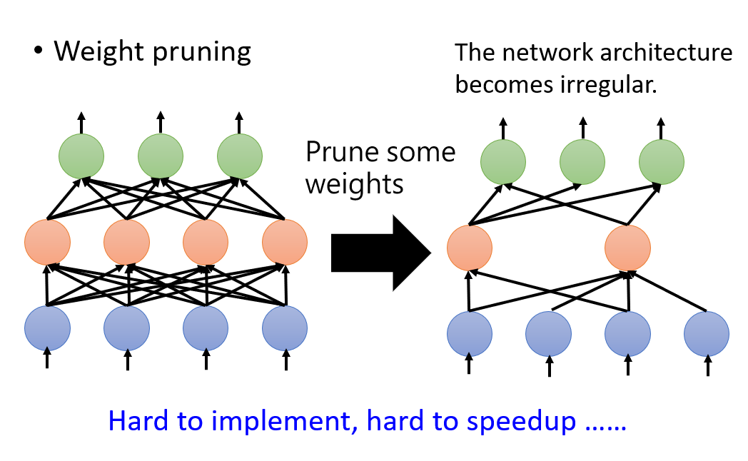
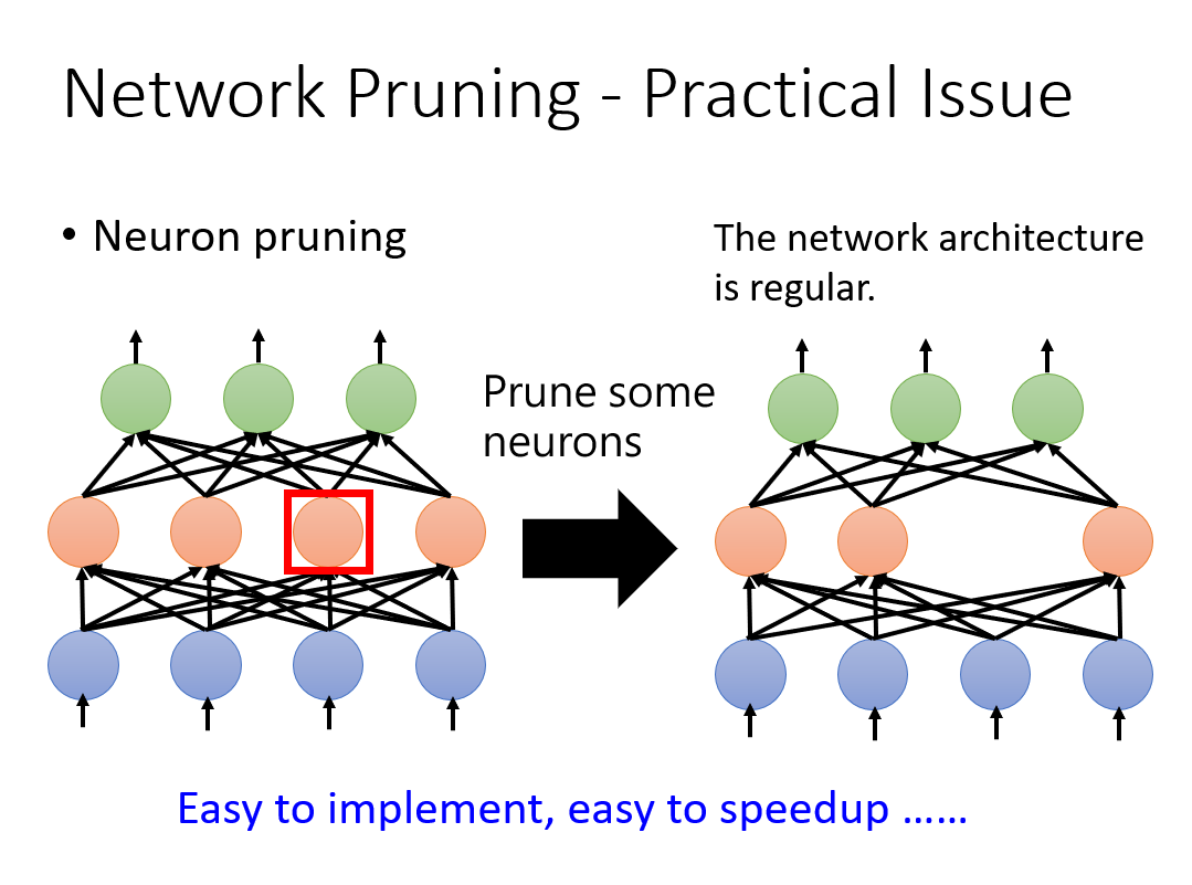
The pruning of neural network is mainly completed from two angles:

• Importance of weight
• The importance of neurons

The importance of weight can be described by common L1 or L2 norm; The importance of neurons can be determined by the number of times that the neuron is not zero in a given data set. (when you think about it, it's similar to the pruning of a decision tree.). From the following two pictures, we can also see the difference between the two pruning methods. Usually, in order to make our network better, we choose to prune according to the importance of neurons.

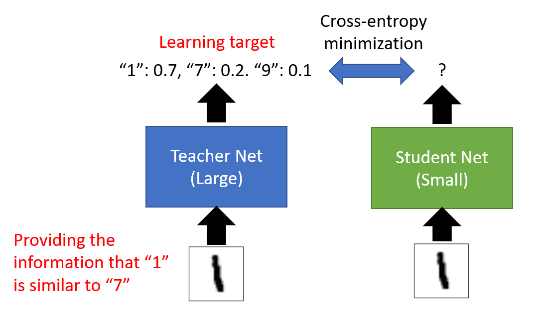
1.2 Knowledge Distillation

Knowledge differentiation is to train a small network to simulate the output of the trained large network. As shown in the figure below, the output of a small network should be consistent with that of a large network. We usually measure the consistency by the loss of cross entropy.

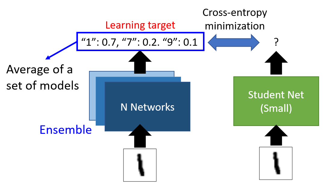
Sometimes, we will let small networks simulate the integration results of a group of large networks. The specific operation is shown in the figure below:

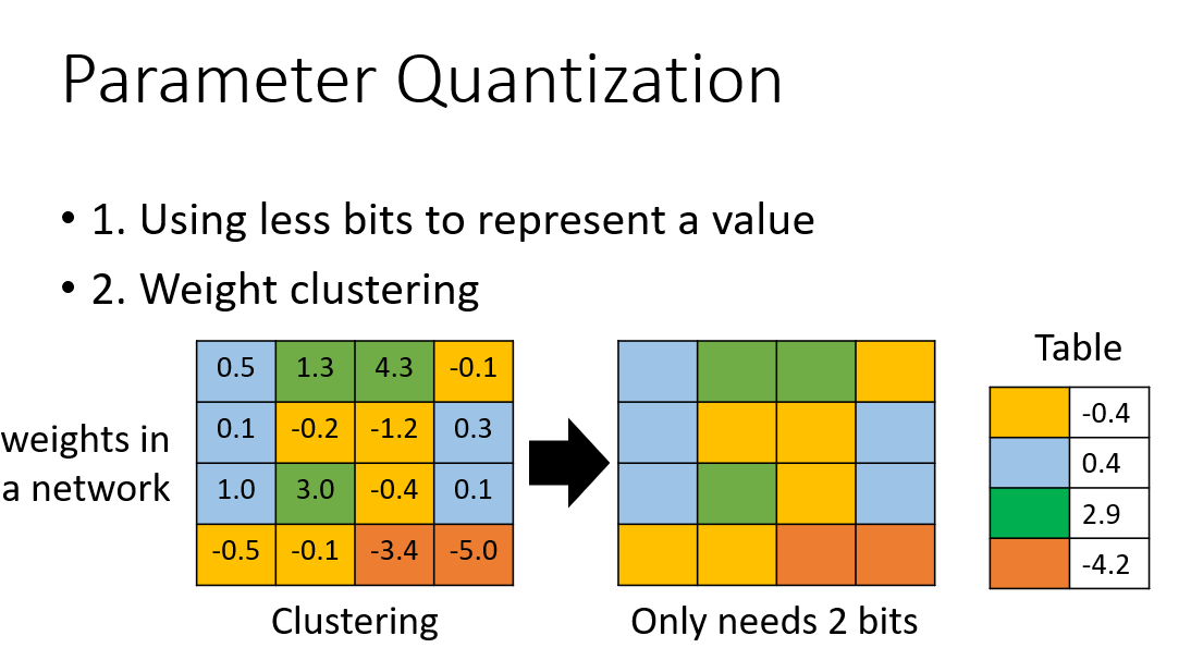
1.3 Parameter Quantization

The main idea of parameter quantification is to use the clustering method to gather similar weights together, and uniformly use a value to replace them. As shown in the figure below:

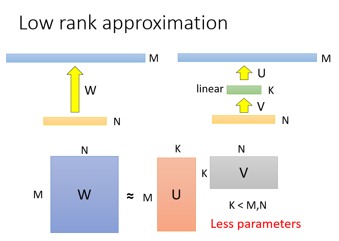
1.4 Architec Design

Architect design changes the network structure to greatly reduce the network parameters. Let's start with an example. This example is a bit like SVD in matrix decomposition, for a N × M N \times M N × M's full connection layer, we add another one with a length of K K K linear layer to achieve the purpose of reducing parameters. We can approximately think of this operation as N × M N \times M N × Matrix of M N × K N \times K N × K and K × M K \times M K × M is replaced by the product of two matrices when K K K is much less than M M M and N N N, the reduction of parameters is obvious.

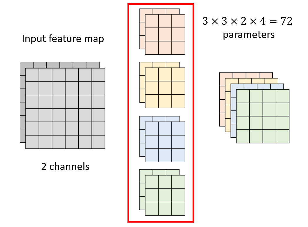
For our common CNN network, as shown in the image of two channels in the figure below, the general convolution operation is to use a convolution core of two channels for convolution every time. After the operation of pink convolution core, a pink matrix is obtained, and after the operation of yellow convolution core, a yellow matrix is obtained, and so on.

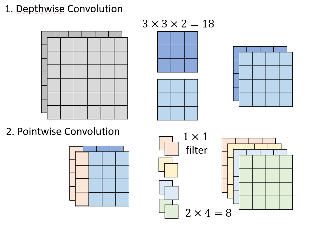
For architect design, the combination of depthwise revolution and pointwise revolution is usually used to achieve the above convolution effect. The specific operations of the two are shown in the figure below: (the results after convolution are obtained by convolution kernels of the same color after convolution operation)

2. Pytoch code

The following code simplifies CNN network using the idea of architect design. The experimental results show that the simplified effect is good.
Depthwise revolution and pointwise revolution can be implemented through the following code:

# General revolution, weight size = in_chs * out_chs * kernel_size^2
nn.Conv2d(in_chs, out_chs, kernel_size, stride, padding)

# Depthwise revolution, input CHS = output CHS = number of groups, weight size = in_chs * kernel_size^2
nn.Conv2d(in_chs, out_chs=in_chs, kernel_size, stride, padding, groups=in_chs)

# Pointwise revolution, i.e. 1 by 1 revolution, weight = in_chs * out_chs
nn.Conv2d(in_chs, out_chs, 1)

The network code is as follows:

import torch.nn as nn
import torch.nn.functional as F
import torch

class StudentNet(nn.Module):
    '''
      In this Net Inside, we'll use it Depthwise & Pointwise Convolution Layer solve model. 
      You will find that the original Convolution Layer change into Dw & Pw After, Accuracy Usually not much.

      In addition, it is named StudentNet Because of this Model You can do it later Knowledge Distillation. 
    '''

    def __init__(self, base=16, width_mult=1):
        '''
          Args:
            base: this model At the beginning ch Quantity, each layer will*2，until base*16 until.
            width_mult: For the future Network Pruning Use, in base*8 chs of Layer Meeting * width_mult Represents after pruning ch quantity        
        '''
        super(StudentNet, self).__init__()
        multiplier = [1, 2, 4, 8, 16, 16, 16, 16]

        # bandwidth: the number of ch used by each Layer
        bandwidth = [ base * m for m in multiplier]

        # We only Pruning the Layer after the third Layer
        for i in range(3, 7):
            bandwidth[i] = int(bandwidth[i] * width_mult)

        self.cnn = nn.Sequential(
            # For the first time, we usually don't disassemble the revolution layer.
            nn.Sequential(
                nn.Conv2d(3, bandwidth[0], 3, 1, 1),
                nn.BatchNorm2d(bandwidth[0]),
                nn.ReLU6(),
                nn.MaxPool2d(2, 2, 0),
            ),
            # Next, each Sequential Block is the same, so we only talk about Block
            nn.Sequential(
                # Depthwise Convolution
                nn.Conv2d(bandwidth[0], bandwidth[0], 3, 1, 1, groups=bandwidth[0]),
                # Batch Normalization
                nn.BatchNorm2d(bandwidth[0]),
                # ReLU6 is the limit of Neuron. The minimum will only be 0 and the maximum will only be 6. MobileNet series all use ReLU6.
                # The reason for using ReLU6 is that if the number is too large, it will not be easy to press to float16 / or further quantization, so it is limited.
                nn.ReLU6(),
                # Pointwise Convolution
                nn.Conv2d(bandwidth[0], bandwidth[1], 1),
                # There is no need to do ReLU after using pointwise revolution. Empirically, the effect of Pointwise + ReLU will become worse.
                nn.MaxPool2d(2, 2, 0),
                # Down Sampling after each Block
            ),

            nn.Sequential(
                nn.Conv2d(bandwidth[1], bandwidth[1], 3, 1, 1, groups=bandwidth[1]),
                nn.BatchNorm2d(bandwidth[1]),
                nn.ReLU6(),
                nn.Conv2d(bandwidth[1], bandwidth[2], 1),
                nn.MaxPool2d(2, 2, 0),
            ),

            nn.Sequential(
                nn.Conv2d(bandwidth[2], bandwidth[2], 3, 1, 1, groups=bandwidth[2]),
                nn.BatchNorm2d(bandwidth[2]),
                nn.ReLU6(),
                nn.Conv2d(bandwidth[2], bandwidth[3], 1),
                nn.MaxPool2d(2, 2, 0),
            ),

            # So far, because the picture has been used by the Down Sample many times, MaxPool is not done
            nn.Sequential(
                nn.Conv2d(bandwidth[3], bandwidth[3], 3, 1, 1, groups=bandwidth[3]),
                nn.BatchNorm2d(bandwidth[3]),
                nn.ReLU6(),
                nn.Conv2d(bandwidth[3], bandwidth[4], 1),
            ),

            nn.Sequential(
                nn.Conv2d(bandwidth[4], bandwidth[4], 3, 1, 1, groups=bandwidth[4]),
                nn.BatchNorm2d(bandwidth[4]),
                nn.ReLU6(),
                nn.Conv2d(bandwidth[5], bandwidth[5], 1),
            ),

            nn.Sequential(
                nn.Conv2d(bandwidth[5], bandwidth[5], 3, 1, 1, groups=bandwidth[5]),
                nn.BatchNorm2d(bandwidth[5]),
                nn.ReLU6(),
                nn.Conv2d(bandwidth[6], bandwidth[6], 1),
            ),

            nn.Sequential(
                nn.Conv2d(bandwidth[6], bandwidth[6], 3, 1, 1, groups=bandwidth[6]),
                nn.BatchNorm2d(bandwidth[6]),
                nn.ReLU6(),
                nn.Conv2d(bandwidth[6], bandwidth[7], 1),
            ),

            # Here we use Global Average Pooling.
            # If the size of the input image is different, it will become the same shape because of the global average pool, so the FC will not be sorry for the next step.
            nn.AdaptiveAvgPool2d((1, 1)),
        )
        self.fc = nn.Sequential(
            # Here we output the answer directly to the 11th dimension.
            nn.Linear(bandwidth[7], 11),
        )

    def forward(self, x):
        out = self.cnn(x)
        out = out.view(out.size()[0], -1)
        return self.fc(out)