1 logistic regression
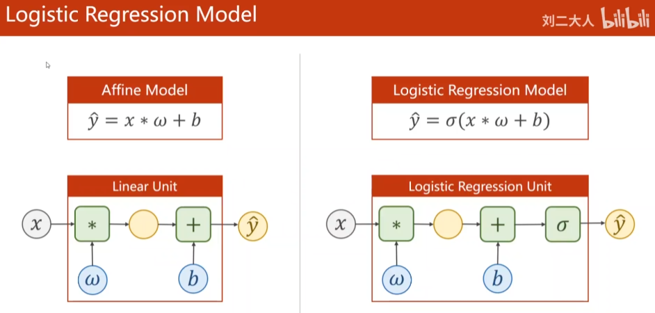
The classification function called regression outputs a probability in the classification problem
Import database
import torchvision
train_set = torchvision.datasets.MNIST(root='../dataset/mnist',train=True,download=True)
test_set = torchvision.datasets.MNIST(root='../dataset/mnist',train=False,download=True)
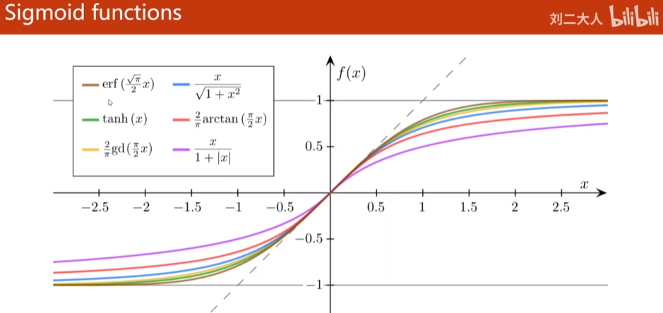
The above figures are sigmoid functions that satisfy: (1) the function has a limit; (2) monotonic increasing function; (3) saturation function (the corresponding derivative is normal distribution), of which the most typical is logistic function (logistic regression), so it is also called sigmoid function
https://en.wikipedia.org/wiki/Logistic_function
∂
(
x
)
=
1
1
+
e
−
x
\partial (x) = \frac {1} {1+e^{-x}}
∂(x)=1+e−x1
Problems in deep learning
∂
\partial
∂ generally refers to logistic function
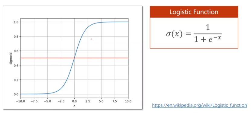
The logistic function maps real numbers between 0 and 1
1.1 logistic regression model
1.2 BCE loss
Compare the differences between the two distributions
Where the value of true value Y is 0 or 1
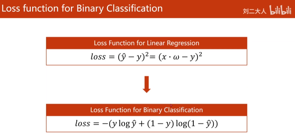
Formula:
l
o
s
s
=
−
(
y
l
o
g
y
^
+
(
1
−
y
)
l
o
g
(
1
−
y
^
)
)
loss = -(ylog \hat y+(1-y)log(1-\hat y))
loss=−(ylogy^+(1−y)log(1−y^))
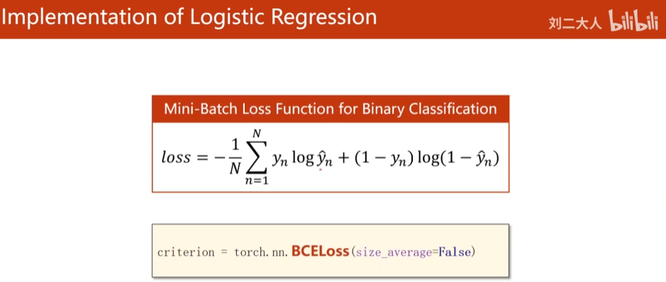
Formula:
l
o
s
s
=
−
1
N
∑
n
=
1
N
y
n
l
o
g
y
^
n
+
(
1
−
y
n
)
l
o
g
(
1
−
y
^
n
)
loss = -\frac {1}{N}\sum ^{N}_{n=1}y_nlog \hat y_n+(1-y_n)log(1-\hat y_n)
loss=−N1n=1∑Nynlogy^n+(1−yn)log(1−y^n)
1.3 complete code
"""
2021.08.04
author:alian
06 Logistic regression
"""

import torch
import torch.nn.functional as F
import torchvision
train_set = torchvision.datasets.MNIST(root='../dataset/mnist',train=True,download=True)
test_set = torchvision.datasets.MNIST(root='../dataset/mnist',train=False,download=True)
# 1. Prepare data set
x_data = torch.Tensor([[1.0],[2.0],[3.0]])
y_data = torch.Tensor([[0],[0],[1]])

# 2. Constructor
class LogisticRegressionModel(torch.nn.Module):
    def __init__(self):  # initialization
        super(LogisticRegressionModel,self).__init__()
        self.linear = torch.nn.Linear(1,1)  # Construct objects, including weights w and offsets b

    def forward(self,x):  # Feedforward is the calculation to be performed
        y_pred = F.sigmoid(self.linear(x)) # 1. Add nonlinear transformation
        return  y_pred

model = LogisticRegressionModel()
# 3. Construct loss function and optimizer
criterion = torch.nn.BCELoss(size_average=False)  # 2. MSE loss becomes BCE loss
optimizer = torch.optim.SGD(model.parameters(),lr=0.01)
# 4. Training cycle
for epoch in range(100):
    y_pred = model(x_data)
    loss = criterion(y_pred,y_data)
    print(epoch,loss)

    optimizer.zero_grad()  # Gradient zeroing
    loss.backward()  # Loss back propagation
    optimizer.step()  # Weight update

# Result test
import numpy as np
import matplotlib.pyplot as plt

x = np.linspace(0,10,200)
x_t = torch.Tensor(x).view((200,1))  # reshape
y_t = model(x_t)
y = y_t.data.numpy()  # Get value
plt.plot(x,y)
plt.plot([0,10],[0.5,0.5],c='r')
plt.xlabel('Hours')
plt.ylabel('Probability of Pass')
plt.grid()
plt.show( )
2 processing multidimensional feature input
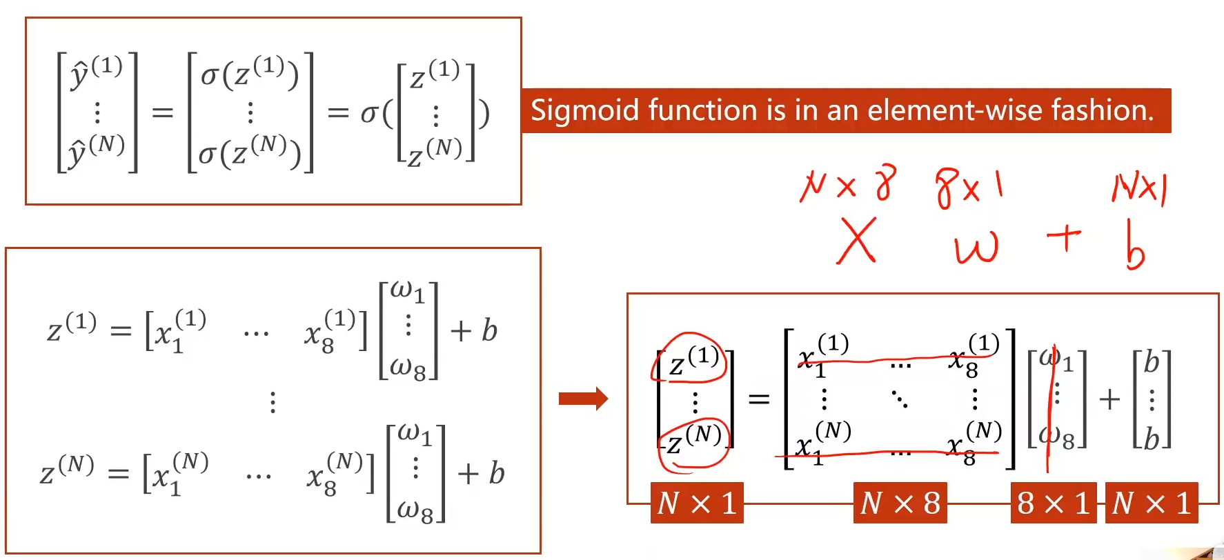
2.1 multidimensional input calculation understanding diagram (vector)
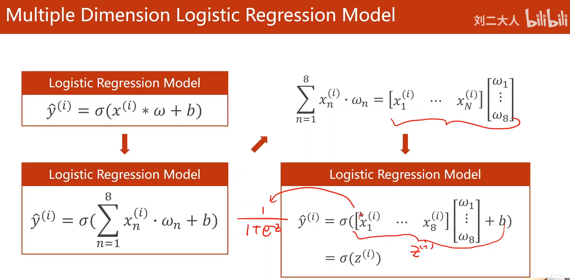
The sigmoid function provided by pytorch is calculated in the form of vector, which is very similar to numpy
Advantages of matrix computing: the equation operation is converted into matrix operation, and the vectorization operation can take advantage of the parallel operation ability of GPU to improve the operation speed
Transformation principle of input and output in matrix space (as shown below):
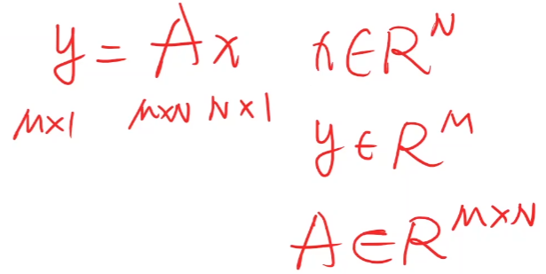
X is mapped from N-dimensional space to m-dimensional space through the linear transformation of an M*N matrix.
However, the spatial transformation we often do is not necessarily linear, but may be very complex and nonlinear. Therefore, we want to use multiple linear transformation layers to simulate this nonlinear transformation by finding the optimal weight and adding nonlinear activation. Therefore, the essence of using convolutional neural network is to find a nonlinear spatial transformation function.
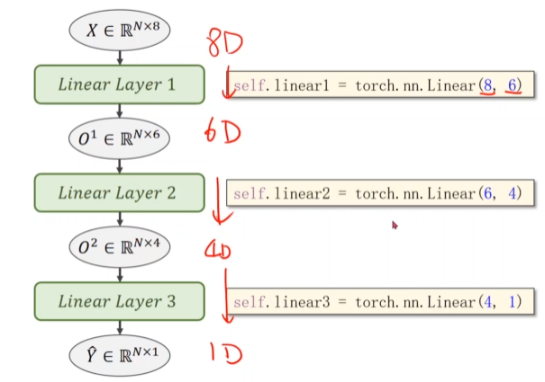
2.2 linking multiple linear layers
The linear layer can realize dimension conversion between input and output of different dimensions
Complete code
"""
2021.08.05
author:alian
07 Processing the input of multidimensional features
"""
import torch
import numpy as np
# 1. Prepare data set
xy = np.loadtxt('diabets.csv.gz',delimiter=',',dtype=np.float32)
x_data = torch.from_numpy(xy[:,:-1])
y_data = torch.from_numpy(xy[:,[-1]])  # [] ensure that the vector is taken out

# 2. Constructor (multiple linear layers)
class Model(torch.nn.Module):
    def __init__(self):  # initialization
        super(Model,self).__init__()
        # Multilayer linear layer
        self.linear1 = torch.nn.Linear(8, 6)  # The input is 8 dimensions and the output is 6 dimensions
        self.linear2 = torch.nn.Linear(6, 4)
        self.linear3 = torch.nn.Linear(4, 1)
        # nn.functionl.sigmoid (function) NN Sigmoid () is a module with the same functions
        self.sigmoid = torch.nn.Sigmoid()  # Activation function, in order to add nonlinear transformation to the linear model

    def forward(self,x):  # Feedforward is the calculation to be performed
        x = self.sigmoid(self.linear1(x))
        x = self.sigmoid(self.linear2(x))
        x = self.sigmoid(self.linear3(x))
        return x
model = Model()
# 3. Construction loss and optimizer

criterion = torch.nn.BCELoss(size_average=True)
optimizer = torch.optim.SGD(model.parameters(),lr=0.01)

# 4. Training cycle
for epoch in range(100):
    y_pred = model(x_data)
    loss = criterion(y_pred,y_data)
    print(epoch,loss.item())

    optimizer.zero_grad()  # Gradient zeroing
    loss.backward()  # Loss back propagation
    optimizer.step()  # Weight update
2.3 various activation functions
http://rasbt.github.io/mlxtend/user_guide/general_concepts/activation-functions/#activation-functions-for-artificial-neural-networks
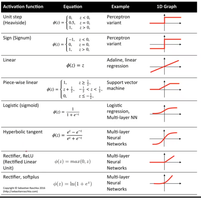
See what the active function looks like
https://dasheeB7.github.io/data#20science/deep#20learning/visualising-activation-functions-in-neural-networks/
View the documentation information of the pytorch activation function
https://pytorch.org/docs/stable/nn.html#non-linear-activations-weighted-sum-nonlinearity
3. Data set loading
3.1 understand epoch, batch size, iterations
- Epoch: all training samples are subject to a process of forward propagation and back propagation
- Batch size: the number of samples used for one feedforward + backpropagation + parameter update
- Iterations: iterations = all samples / batch size
3.2 use of dataloader (batch_size = 2, shuffle = true)
DataLoader: you need to know the sample length of the dataset and its index
Shuffle: shuffle data sets
"""
2021.08.05
author:alian
08 Load dataset
"""
import torch
from torch.utils.data import Dataset,DataLoader
import numpy as np

# Custom dataset
class DiabetesDataset(Dataset):
    def __init__(self,filepath):
        xy = np.loadtxt(filepath, delimiter=',', dtype=np.float32)  # The data path, with "," as the separator, reads the 32-bit sequence
        self.len = xy.shape[0]  # Get data length
        self.x_data = torch.from_numpy(xy[:, :-1])  # Read the first 8 columns
        self.y_data = torch.from_numpy(xy[:, [-1]])  # Read the last column, [] make sure that the vector is taken out

    def __getitem__(self, index):
        return self.x_data[index],self.y_data[index]  # Get data index

    def __len__(self):
        return self.len

dataset = DiabetesDataset('diabets.csv.gz')  # Incoming path
# With a batch_ The data set is loaded according to the data volume of size
train_loder = DataLoader(dataset=dataset,
                         batch_size=32,
                         shuffle=True,
                         num_workers=2)

# 2. Constructor (multiple linear layers)
class Model(torch.nn.Module):
    def __init__(self):  # initialization
        super(Model,self).__init__()
        self.linear1 = torch.nn.Linear(8, 6)  # The input is the 8 dimension and the output is the 1 dimension
        self.linear2 = torch.nn.Linear(6, 4)
        self.linear3 = torch.nn.Linear(4, 1)
        self.sigmoid = torch.nn.Sigmoid()

    def forward(self,x):  # Feedforward is the calculation to be performed
        x = self.sigmoid(self.linear1(x))
        x = self.sigmoid(self.linear2(x))
        x = self.sigmoid(self.linear3(x))
        return x
model = Model()

# 3. Construction loss and optimizer

criterion = torch.nn.BCELoss(size_average=False)
optimizer = torch.optim.SGD(model.parameters(),lr=0.01)

# 4. Training cycle
for epoch in range(100):
    for i, data in enumerate(train_loder,0):  # An iteration
        # 1. Prepare data
        input,labels = data
        # 2. Forward
        y_pred = model(input)
        loss = criterion(y_pred,labels)  # Calculate loss
        print(epoch,loss.item())
        # 3.Backward
        optimizer.zero_grad()  # Gradient zeroing
        loss.backward()  # Loss back propagation
        # 4. Update
        optimizer.step()  # Weight update
3.3 num_workers in Windows
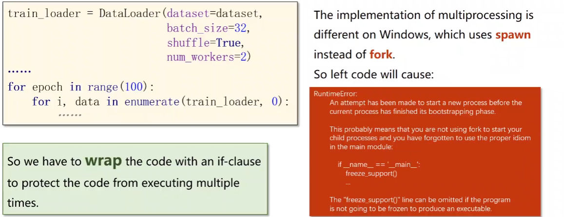
Problem solving: encapsulate the cyclic code containing DataLoder instead of calling it in the main program.

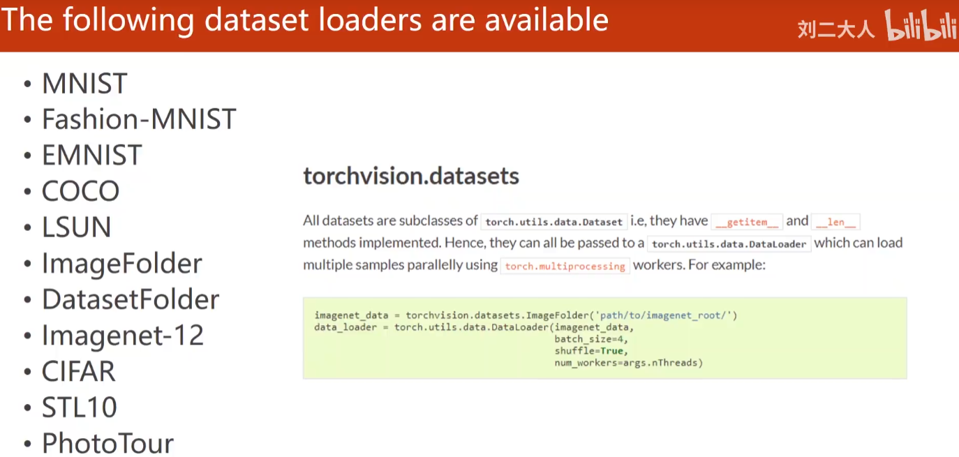
3.4 torchvision built-in dataset (loadable)
# Load built-in dataset
import torch
from torch.utils.data import DataLoader
from torchvision import datasets,transforms

train_dataset = datasets.MNIST(root='../dataset/mnist',  # route
                               train=True,
                               transform=transforms.ToTensor(),  # Image conversion to tensor
                               download=True)  # Download online

test_dataset = datasets.MNIST(root='../dataset/mnist',
                               train=False,
                               transform=transforms.ToTensor(),  # Image conversion to tensor
                               download=True)
# Data loading to batch_size (due to hardware limitations, all data cannot be loaded at one time)
train_loder = DataLoader(dataset=train_dataset,
                         batch_size=32,
                         shuffle=True)
test_loder = DataLoader(dataset=train_dataset,
                         batch_size=32,
                         shuffle=False)
for batch_idx,(inputs, target) in enumerate(train_loader):
3.5 practice
Training objective: does the passenger survive
https://www.kaggle.com/c/titanic/data

4 multi classification problem
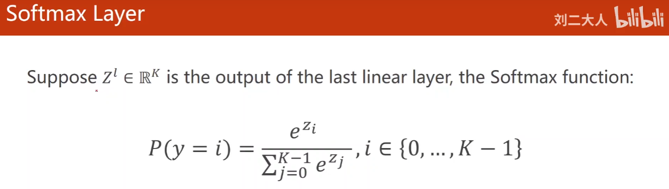
4.1 how does softmax classifier solve multi classification problems
Distribution: probability of belonging to each category
Multi classification problems need to meet:
- P ( y = i ) ≥ 0 P(y=i)\geq 0 P(y=i)≥0
- ∑ i = 0 N P ( y = i ) = 1 \sum ^N_{i=0}{P(y=i)=1} ∑i=0NP(y=i)=1
The Softmax function meets the appeal requirements:
P
(
y
=
i
)
=
e
Z
i
∑
j
=
0
K
−
1
e
Z
j
,
i
∈
(
0
,
.
.
.
,
K
−
1
)
P(y=i)=\frac {e^{Z_i}}{\sum ^{K-1}_{j=0}{e^{Z_j}}},i\in (0,...,K-1)
P(y=i)=∑j=0K−1eZjeZi,i∈(0,...,K−1)
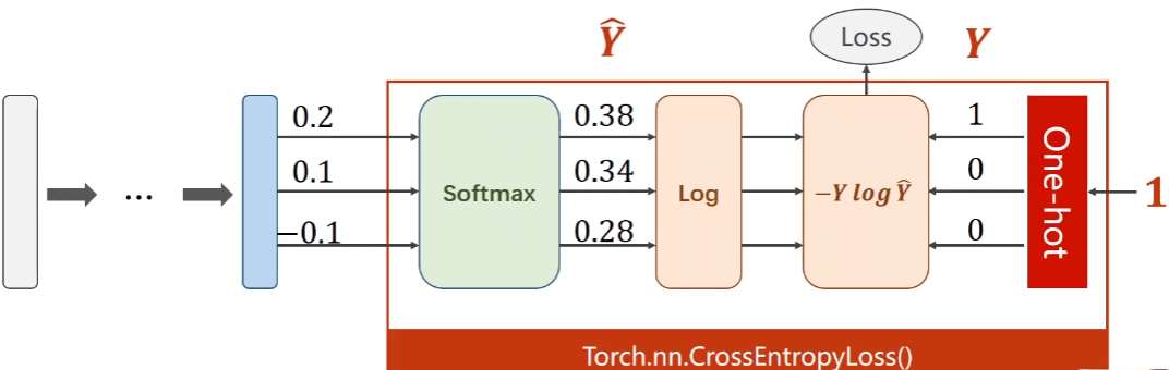
4.2 loss function of multi classification: cross entropy loss
The cross entropy loss based on binary classification is extended. The truth Y is one hot distribution, the real category is 1, and the other categories are 0
(1) Multi classification cross entropy based on numpy
import numpy as np
y = np.array([1,0,0])
z = np.array([0.2,0.1,-0.1])
y_pred = np.exp(z)/np.exp(z).sum()
loss = (-y*np.log(y_pred)).sum()
print(loss)
(2) Implementation of multi classification cross entropy with pytorch
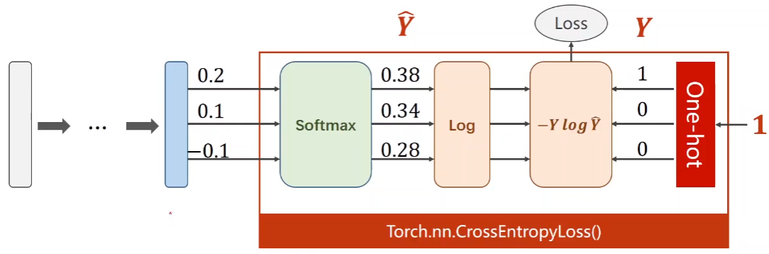
# Multi classification cross entropy loss based on pytorch
y = torch.LongTensor([0])
z = torch.Tensor([[0.2,0.1,-0.1]])
criterion = torch.nn.CrossEntropyLoss()
loss = criterion(z,y)
print(loss)
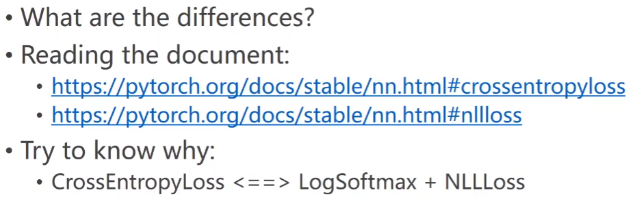
practice
https://pytorch.org/docs/stablr/nn.html#crossentropyloss
https://pytorch.org/docs/stablr/nn.html#nllloss
4.3 pytorch realizes multi classification training
4.3. 1 data preparation
import torch
from torchvision import transforms,datasets
from torch.utils.data import DataLoader
import torch.nn.functional as F
import torch.optim as optim
# 1. Data set preparation
batch_size = 64
# transforms:
# (1) Map the image pixel value (image tensor) to 0-1
# (2)H*W*C into C*H*W
# (3)Normalize, normalize (mean, standard deviation) to meet the 0-1 distribution
transform = transforms.Compose([
    transforms.ToTensor(),
    transforms.Normalize((0.1307,),(0.3081,))
])

train_dataset = datasets.MNIST(root='../dataset/mnist',
                               train=True,
                               transform=transforms.ToTensor(),  # Image conversion to tensor
                               download=True)

test_dataset = datasets.MNIST(root='../dataset/mnist',
                               train=False,
                               transform=transforms.ToTensor(),  # Image conversion to tensor
                               download=True)
train_loder = DataLoader(dataset=train_dataset,
                         batch_size=32,
                         shuffle=True)
test_loder = DataLoader(dataset=train_dataset,
                         batch_size=32,
                         shuffle=False)
Data normalization: (mean, standard deviation)
P
i
x
e
l
n
o
r
m
=
P
i
x
e
l
o
r
i
g
i
n
−
m
e
a
n
s
t
d
Pixel_{norm} = \frac {Pixel_{origin}-mean}{std}
Pixelnorm=stdPixelorigin−mean
4.3. 2 model design
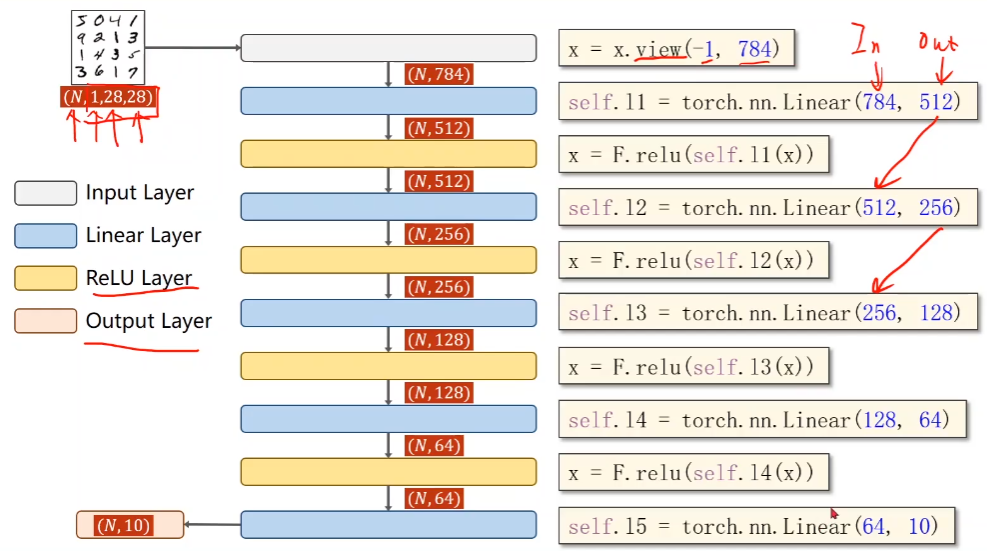
# 2. Design model
class Net(torch.nn.Module):
    def __init__(self):
        super(Net,self).__init__()
        self.l1 = torch.nn.Linear(784,512)
        self.l2 = torch.nn.Linear(512, 256)
        self.l3 = torch.nn.Linear(256, 128)
        self.l4 = torch.nn.Linear(128, 64)
        self.l5 = torch.nn.Linear(64, 10)

    def forward(self,x):
        x = x.view(-1,784)
        x = F.relu(self.l1(x))
        x = F.relu(self.l2(x))
        x = F.relu(self.l3(x))
        x = F.relu(self.l4(x))
        return self.l5(x)
model = Net()
4.3. 3 construction loss and optimizer
# 3. Construct loss function and optimizer
criterion = torch.nn.CrossEntropyLoss()
optimizer = optim.SGD(model.parameters(),lr=0.01,momentum=0.5)  # Optimizer (with impulse, 0.5)
4.3. 4 training cycle
Define single round epoch as a function
def train(epoch):
    running_loss = 0.0
    for batch_idx,data in enumerate(train_loder,0):
        inputs,target = data
        optimizer.zero_grad()

        # forward+backward+updata
        output = model(inputs)
        loss = criterion(output,target)
        loss.backward()
        optimizer.step()

        running_loss+=loss.item()
        if batch_idx % 300 == 299:
            print('[%d,%5d] loss: %.3f' % (epoch+1, batch_idx+1,running_loss/300))
            running_loss = 0.0
4.3. 5 complete code
"""
2021.08.05
author:alian
09 Multi classification problem
"""
import torch
from torchvision import transforms,datasets
from torch.utils.data import DataLoader
import torch.nn.functional as F
import torch.optim as optim

# 1. Data set preparation
batch_size = 64
# transforms:
# (1) Map the image pixel value (image tensor) to 0-1
# (2)H*W*C into C*H*W
# (3)Normalize, normalize (mean, standard deviation) to meet the 0-1 distribution
transform = transforms.Compose([
    transforms.ToTensor(),
    transforms.Normalize((0.1307,),(0.3081,))
])

train_dataset = datasets.MNIST(root='../dataset/mnist',
                               train=True,
                               transform=transforms.ToTensor(),  # Image conversion to tensor
                               download=True)

test_dataset = datasets.MNIST(root='../dataset/mnist',
                               train=False,
                               transform=transforms.ToTensor(),  # Image conversion to tensor
                               download=True)
train_loder = DataLoader(dataset=train_dataset,
                         batch_size=32,
                         shuffle=True)
test_loder = DataLoader(dataset=train_dataset,
                         batch_size=32,
                         shuffle=False)
# 2. Design model
class Net(torch.nn.Module):
    def __init__(self):
        super(Net,self).__init__()
        self.l1 = torch.nn.Linear(784,512)
        self.l2 = torch.nn.Linear(512, 256)
        self.l3 = torch.nn.Linear(256, 128)
        self.l4 = torch.nn.Linear(128, 64)
        self.l5 = torch.nn.Linear(64, 10)

    def forward(self,x):
        x = x.view(-1,784)
        x = F.relu(self.l1(x))
        x = F.relu(self.l2(x))
        x = F.relu(self.l3(x))
        x = F.relu(self.l4(x))
        return self.l5(x)
model = Net()

# 3. Construct loss function and optimizer
criterion = torch.nn.CrossEntropyLoss()
optimizer = optim.SGD(model.parameters(),lr=0.01,momentum=0.5)

# 4. Training cycle
def train(epoch):
    running_loss = 0.0
    for batch_idx,data in enumerate(train_loder,0):
        inputs,target = data
        optimizer.zero_grad()

        # forward+backward+updata
        output = model(inputs)
        loss = criterion(output,target)
        loss.backward()
        optimizer.step()

        running_loss+=loss.item()
        if batch_idx % 300 == 299:
            print('[%d,%5d] loss: %.3f' % (epoch+1, batch_idx+1,running_loss/300))
            running_loss = 0.0
# test
def test():
    correct = 0
    total = 0
    with torch.no_grad():  # The gradient does not need to be calculated
        for data in test_loder:
            images,labels = data
            outputs = model(images)
            _, predicted = torch.max(outputs.data, dim=1)
            total +=labels.size(0)
            correct += (predicted == labels).sum().item()
    print('Accurary on test set: %d %%' % (100 * correct/total))

if __name__ == '__mian__':
    for epoch in range(10):
        train(epoch)
        test()