1, Install Anaconda

Download from the official website, select the installation location, select all user, select the configuration environment, and install the rest next.

2, Create virtual environment

1. Open Anaconda Prompt
2. To create a virtual environment, enter:

conda create --name pytorch python=3.8

Where pytorch is the name of the virtual environment.
3. Enter the virtual environment and enter:

conda activate pytorch

Note: the command to close the virtual environment is as follows:

conda deactivate

Delete:

conda remove -n Environment name --all

Add package:

conda install -n Environment name package name

Remove package:

conda remove -n Environment name package name

1. After entering the virtual environment, you can install pytorch and enter the official website( https://pytorch.org/ ), click Get Start to enter the download, and select the following:
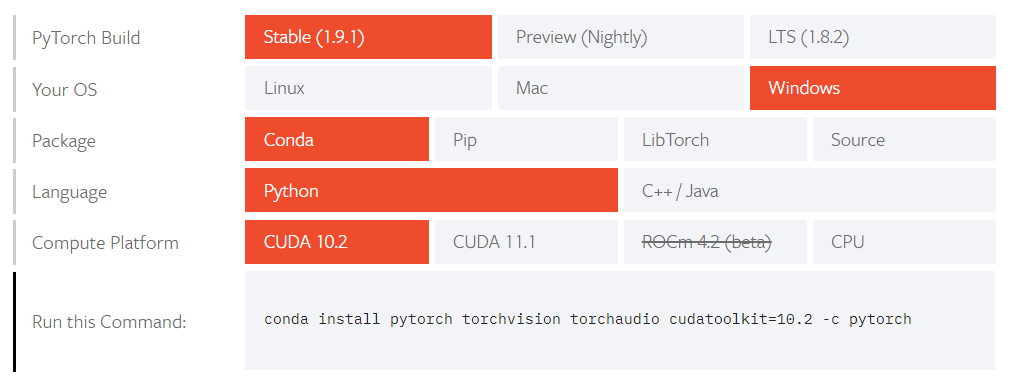
   run this command is the required command, which can be entered in pytorch.
   Note that for the GPU Version (which requires hardware support, you can drop down on the left in Task Manager - > performance. If the GPU description support is displayed, there is a large difference between the speed of the complex neural network and the CPU version, and there is no difference in the rest), CUDA and cudnn need to be installed first( Installation tutorial ), it is recommended to install the GPU version. Pay attention to CUDA version! Mainly consistent with your own computer version! (the pro test can be inconsistent with that in the virtual environment. Cuda11.0 + CUDA10.2 of pytoch succeeded)
2. To install Jupyter, enter:

conda install jupyter

1. You can also use the conda command to install other Python libraries you need.
2. Verification: you can open Anaconda Navigator, select pytorch in the Applications on drop-down list box of the interface, and then start jupyter notebook in this environment( Using tutorials ), enter the import statement. If no error is reported, it indicates that PyTorch has been successfully installed. You can also view the installed version of PyTorch in Jupyter Notebook (note that there are two underscores).
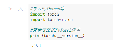
   Torch is the core library of python, and torch vision package serves the deep learning framework to generate pictures, video data sets, some popular model classes and pre training models.

3, Tensor

1. Tensor is the basic operation unit in pytorch, which is similar to the array in numpy, but only tensor can run on GPU version of pytorch, so it is faster.
2. Creation of tensor:
   1. Randomly initialized tensor:

      x = torch.randn(2,2)
      

   2. Create tensor from Python list:

      x = torch.tensor([1,2],[3,4])
      

   3. Create an all zero tensor:

      x = torch.zeros(2,2)
      

   4. Create an all one tensor:

      x = torch.ones(2,2)
      

   5. Create a new tensor based on an existing tensor:

      y= torch.ones_like(x)
      

   6. Create a tensor of the specified data type:

      x = torch.ones(2, 2, dtype=torch.long)
      

3. Mathematical operation of tensor: the same as that of array.
   1. Add two tensors:
      1. You can use '+' to add directly.
      2. You can use torch.add() to add tensors and assign values to variables for storage.
      3. You can also use. add_ () realize the substitution of tensors.

         z = x + y
         w = torch.add(x, y)
         #Save and to y:
         y.add_(x)
         

   2. Tensor multiplication:
      1. Multiply corresponding elements by. mul():

         x = torch.tensor([[1,2],[3,4]])
         y = torch.tensor([[1,2],[3,4]])
         x.mul(y)
         #Results obtained:
         #[[1,4],
         #[9,16]]
         

      2. Matrix multiplication (mm):

         x = torch.tensor([[1,2],[3,4]])
         y = torch.tensor([[1,2],[3,4]])
         x.mm(y)
         #Results obtained:
         #[[7,10],
         #[15,22]]
         

4. Transformation of tensor and NumPy array:
   1. Convert tensor to NumPy array, using. numpy().

y = x.numpy()
#You can view the current type:
print(type(y))

2. Convert numpy array to tensor and use torch.from_numpy().

y = torch.from_numpy(x)

1. CUDA tensor: the newly created tensor is saved in the CPU by default. PyTorch with GPU version installed can be moved to the GPU.

   a = torch.ones(2,2)
   if torch.cuda.is_available():
   	a_cuda = a.cuda()

4, Automatic derivation

1. The essence of deep learning algorithm is to find the derivative through back propagation, which is realized by PyTorch's automatic derivation module. For all operations of tensor, the automatic derivation module can automatically provide differentiation for it.
2. There is no automatic derivation function for tensors by default. If you want tensors to use the automatic derivation function, you need to set the parameter 'tensor. Requires' when defining tensors_ grad=True’.

x = torch.ones(2, 2, requires_grad = True)
#Can view
print(x.requires_grad)

1. Each variable calculated by the function has a. grad_fn attribute.
2. For z = averaging (x+y) in the following example, to find the partial derivatives of z to X and z to y, first use backward() for z to define back propagation, and then directly use x.grad to calculate the partial derivatives of z to X.

z = x + y
#mean(): Average
z = z.mean()
#Back propagation
z.backward()
#Calculate the partial derivative of z over x
print(x.grad)
#Calculate the partial derivative of z over y
print(y.grad)

1. The above z is a scalar (the scalar is zero dimensional (only the size has no direction), the vector is one-dimensional, the matrix is two-dimensional, and it can be called a tensor no matter how many dimensions). If z is a multi-dimensional tensor, you need to specify parameters (enter a tensor of the same size) in backward() to match the corresponding size.

x = torch.ones(2, 2, requires_grad = True)
y = torch.ones(2, 2, requires_grad = True)
z = 2 * x + 3 * y
#Back propagation
z.backward(torch.ones_like(z))
#Calculate the partial derivative of z over x
print(x.grad)
#Calculate the partial derivative of z over y
print(y.grad)

1. You can use with torch.no_grad() to disable the requirements that have been set_ Tensor of grad = true and retrograde automatic derivation.

with torch.no_grad():
   print(z.requires_grad)
#The output is False

5, Basic framework of torch.nn and torch.optim

1. torch.nn: a modular interface specially designed for neural networks. It is built on the basis of automatic derivation module and can be used to define and run neural networks.
   1. torch.nn is used to build a model, so you need to import this library before use:

import torch
import torch.nn as nn

	2. use torch.nn To build a model, define a class:

#net_name is the class name, which can be drawn up freely. It needs to inherit the parent class nn.Module
#nn.Module class is a very important class in torch.nn, which contains the definitions of network layers and forward methods to avoid the trouble of building the network from the bottom
class net_name(nn.Module): 
	def __init__(self):
		super(net_name, self).__init__()
		#For the construction of the model, the model here is only a full connection layer (fc), also known as the linear layer.
		#The numbers in (1, 1) represent the input and output dimensions respectively. Here, the input and output dimensions are 1.
		self.fc = nn.Linear(1, 1)
		#Other layers
	
	def forward(self, x):
		#Because the model is only a full connection layer, so:
		out = self.fc(x)
		return out

When using the linear regression model, you can directly create an object of the model:

net = net_name()

1. torch.optim: a library that implements various optimization algorithms, including the simplest gradient descent, random gradient descent and other more complex optimization algorithms.
   1. Import torch.optim:

import torch.optim as optim 

	2. PyTorch Loss function in: used to calculate whether the output of each instance is consistent with the real sample label, and evaluate the size of the gap. torch.nn It is very convenient to define the loss function. The simplest is nn.MSELoss()，That is, calculate the mean square error between the pre-test and the real value.

criterion = nn.MSELoss()
#output is the predicted value and target is the real value
loss = criterion(output, target)

	3. In the process of back propagation, common loss.backward()Calculate the gradient. The gradient must be cleared at each iteration, otherwise it will be accumulated.
	4. The simplest optimization algorithm uses the random gradient descent algorithm:

#net.parameters() represents model parameters, i.e. parameters to be calculated
#lr is the learning rate
optimizer = optim.SGD(net.parameters(), lr=0.01)

#In particular, optimizer can specify the learning rate of each layer.

1. Summary: torch.nn and torch.optim packages are required for a complete forward propagation plus back propagation.
   Note: all optimizer s implement the step() method, which will update all parameters. In a single iteration, you only need to call it directly after the gradient is calculated; When the function needs to be calculated repeatedly, you need to pass in a closure to allow them to recalculate your model. This closure should empty the gradient, calculate the loss, and then return.
   Code corresponding to a single iteration:

#The gradient is cleared. Note that the gradient must be cleared before each iteration, otherwise the last gradient will be superimposed
optimizer.zero_grad()

output = net(input)
#Calculate loss
loss = criterion(output, target)
loss.backward()

#Update complete
optimizer.step()

Code corresponding to multiple iterations:

for input, target in dataset:
    def closure():
        optimizer.zero_grad()
        output = net(input)
        loss = criterion(output, target)
        loss.backward()
        return loss
    optimizer.step(closure)

6, Linear regression

The following is an example of linear regression:

1. Basic principle of linear regression: linear regression is generally used for numerical prediction, which is to find such a fitting curve or fitting surface to fit the real data distribution to the greatest extent. We hope that the closer the fitted predicted value is to the real value, the better. Therefore, we introduce a cost function (the smaller the cost function, the better the straight-line fitting). The cost function is defined on the whole training set and is the average of all sample errors, that is, the average of all sample loss functions (the only difference between the two is that the cost function is for the whole training set and the loss function is for a single sample) Therefore, we need to find the corresponding parameters when minimizing the cost function. The method of minimizing the cost function is the gradient descent method: at a certain point on the function curve, the function has the maximum rate of change along the gradient direction, so moving along the negative gradient direction will continue to approach the minimum value.
2. Combined with the above concepts, in this example, the fitting line is y=W0+W1x, and the cost function is calculated through the mean square error: J=1/(2m)(∑ (1 ~ m) (Yi Yi `) ^ 2), where M represents the total number of samples, and the denominator is 2m, just for the convenience of square derivation. In the gradient descent algorithm, W0 and W1 iterate and update the expression: W0=W0- α (J calculates the partial derivative of W0), W1=W1- α (partial derivative of W1), where α Indicates the learning rate.
3. PyTorch implementation of linear regression:
   1. Dataset: build dataset.

   # y=3*x+10, followed by torch.randn() function to make noise
   x = torch.unsqueeze(torch.linspace(-1, 1, 50), dim=1)
   y = 3*x +10 +0.5*torch.randn(x.size())
   

    		Function introduction:
    		1. torch.unsqueeze(input, dim, out=None): Returns a new tensor and inserts dimension 1 into the given position of the input.
    		Note: the return tensor shares memory with the input tensor, so changing the content of one will change the other. If dim If it is negative, it will be converted dim+input.dim()+1
    		Parameters: tensor (Tensor): Input tensor.
    		dim (int): Inserts the index of the dimension.
    		out (Tensor, optional): Result tensor.
    		difference: unsqueeze_ and unsqueeze Achieve the same function,The difference is unsqueeze_ yes in_place operation,Namely unsqueeze Will not be used for unsqueeze of tensor Make changes,Want to get unsqueeze The value after must be given a new value, unsqueeze_ Will change yourself.
    		2. Supplementary introduction: torch.squeeze(input, dim=None, out=None): Dimension reduction, remove 1 from the input tensor shape and return it when given dim When, the extrusion operation is only on a given dimension.
    		Note: the return tensor shares memory with the input tensor, so changing the content of one will change the other.
    		parameter:input (Tensor): Input tensor.
    		dim (int, optional): If given, then input Will only squeeze in a given dimension.
    		out (Tensor, optional): Output tensor.
    		Reason: multidimensional tensor is essentially a transformation. If the dimension is 1, then 1 only plays the role of expanding the dimension without other purposes. Therefore, in order to speed up the calculation, these dimensions of 1 can be removed during dimension reduction.
    		3. torch.linspace(start, end, steps=100, out=None): Returns a 1-dimensional tensor contained in an interval start and end Evenly spaced on step The length of the output tensor is determined by steps decision.
    		Parameters: start (float): The starting point of the interval.
    		end (float): The end of the interval.
    		steps (int): stay start and end Number of samples generated between.
    		out (Tensor, optional): Result tensor.
    2. Model definition: define linear regression model, loss function and optimization function.
   

#Define linear regression model
class LinearRegression(nn.Module):
	def __init__(self):
		super(LinearRegression, self).__init__()
		self.fc = nn.Linear(1, 1)
	def forward(self, x):
		out = self.fc(x)
		return out

model = LinearRegression()   #Instantiation requires parentheses

#Define loss function and optimization function
criterion = nn.MSELoss()
optimizer = optim.SGD(model.parameters(),  lr=5e-3)

	4. Model training: the following is 1000 iterations(Number of times to traverse the entire dataset)The code needs to first propagate forward to calculate the cost function, and then propagate backward to calculate the gradient.
	Forward propagation and back propagation(It will be said in the follow-up notes)

num_epochs = 1000   #Number of times to traverse the training set
for epoch in range(num_epochs):
	#forward
	out = model(x)   #Forward propagation
	loss = criterion(out, y)   #Calculation loss function
	#backward
	optimizer.zero_grad()   #Gradient zeroing
	loss.backward()   #Back propagation
	optimizer.step()   #Update parameters

	5. Model test: Pass model.eval()Function changes the model from training mode to test mode, and puts the data into the model for prediction.

model.eval()
y_hat = model(x)   #Prediction value of trained linear regression model
plt.scatter(x.numpy(), y.numpy(), label='raw data')
#The gradient tracking is required in the model training phase, but not in the model testing phase, so. detach() is required to stop the gradient tracking of tensor
plt.plot(x.numpy(), y_hat.detach().numpy(), c='r', label='Fitting line')
#Show Legend 
plt.legend()
plt.show()

You can view the parameters W0 and W1 of this line:

list(model.name_parameters())

	6. Display of all codes and results:

import torch
import torchvision
import torch.nn as nn
import torch.optim as optim 
from matplotlib import pyplot as plt
import matplotlib

# y=3*x+10, followed by torch.randn() function to make noise
x = torch.unsqueeze(torch.linspace(-1, 1, 50), dim=1)
y = 3*x +10 +0.5*torch.randn(x.size())

#Define linear regression model
class LinearRegression_my(nn.Module):
	def __init__(self):
		super(LinearRegression_my, self).__init__()
		self.fc = nn.Linear(1, 1)
	def forward(self, x):
		out = self.fc(x)
		return out

model_my = LinearRegression_my()

#Define loss function and optimization function
criterion = nn.MSELoss()
optimizer = optim.SGD(model_my.parameters(),  lr=5e-3)

num_epochs = 1000   #Number of times to traverse the training set
for epoch in range(num_epochs):
	#forward
	out = model_my(x)   #Forward propagation
	loss = criterion(out, y)   #Calculation loss function
	#backward
	optimizer.zero_grad()   #Gradient zeroing
	loss.backward()   #Back propagation
	optimizer.step()   #Update parameters
    
model_my.eval()
y_hat = model_my(x)   #Prediction value of trained linear regression model
plt.scatter(x.numpy(), y.numpy(), label='raw data')
#The gradient tracking is required in the model training phase, but not in the model testing phase, so. detach() is required to stop the gradient tracking of tensor
plt.plot(x.numpy(), y_hat.detach().numpy(), c='r', label='Fitting line')
#Show Legend 
plt.legend()
plt.show()

list(model_my.named_parameters())