For an input picture, the picture is a grid image, that is, the picture is divided into one grid, and each grid represents one pixel. For patch (picture block), we traverse the picture from top to bottom and from left to right according to the size of the block, and then convolute each image block.

How to convolute:
(1) For the convolution of a single channel, first draw a 3x3 window in the input image according to the scale of the convolution core, such as 3X3, and then multiply the window with the convolution core, that is, multiply and add the corresponding position elements, and then move the window to traverse continuously to obtain the output. The specification of the output is: (input specification - (convolution core specification-1))
(2) For the convolution of multi-channel pictures, each channel should correspond to a convolution kernel, that is, if the input picture has several channels, the convolution kernel should have several channels; For a multi-channel convolution kernel and a multi-channel picture, the final result can only output a single channel result, so if the final output result is multi-channel, the number of convolution cores is equal to the number of output channels.

Padding
If you want the final convolution and the output image size remains the same, you can add n circles outside the image through Padding. The default method is pixel 0. Generally speaking, if the convolution kernel size is nxn, for example, the picture will be supplemented with n/2 cycles (integer division).

Down sampling:
Convolution neural network needs to combine convolution and down sampling. The most commonly used down sampling is Max pooling. Using down sampling can reduce the data scale. After Max pooling, the number of channels of the picture remains unchanged, but the image size changes.

The network structure of convolutional neural network is realized this time:
The data set of convolutional neural network this time adopts the MNIST image data set in pytoch. After transformation, the image is 1x28x28.
Firstly, we use a convolution layer (convolution core: 5x5) to convert the output image channel into 10 channels, with a scale of 10x24x24;
Then it passes through a 2x2 pool layer, and the image becomes 10x12x12;
After another convolution layer (convolution core: 5x5), the number of channels becomes 20, and the image is 20x8x8;
After a 2x2 pool layer, it becomes 20x4x4;
Finally, the final result is transformed into a 1-dimensional vector through the full connection layer.

Code implementation:

# -*- coding: utf-8 -*-
# @Time : 2022/1/28 14:24
# @Author : CH339
# @FileName: Test1_28_1.py
# @Software: PyCharm
# @Blog : https://blog.csdn.net/weixin_56068397/article/

'''
Convolutional neural network
'''

import torch
from torchvision import transforms
from torchvision import datasets
from torch.utils.data import DataLoader
import torch.nn.functional as F
import torch.optim as optim

batch_size = 64
# Transform the picture into a tensor in pytorch
transform = transforms.Compose([
    # Transform into tensor
    transforms.ToTensor(),
    # Standardize and convert to 0-1 distribution
    transforms.Normalize((0.1307,),(0.3081,))
])
# Construct training set
train_dataset = datasets.MNIST(root='../dataset/mnist/',train=True,download=True,transform=transform)
train_loader = DataLoader(train_dataset,shuffle=True,batch_size=batch_size)

# Construction testing machine
test_dataset = datasets.MNIST(root='../dataset/mnist/',train=False,download=True,transform=transform)
test_loader = DataLoader(test_dataset,shuffle=False,batch_size=batch_size)

# Write model classes
# First, you need to convert c*w*H into a first-order vector
class ConvNet(torch.nn.Module):
    def __init__(self):
        super(ConvNet, self).__init__()
        # Convolution layer
        self.conv1 = torch.nn.Conv2d(1,10,kernel_size=5)
        self.conv2 = torch.nn.Conv2d(10,20,kernel_size=5)
        # Maximum pool layer
        self.pool = torch.nn.MaxPool2d(2)
        # Full connection layer
        self.linear = torch.nn.Linear(320,10)

    def forward(self,x):
        # Get batch
        batch = x.size(0)
        x = F.relu(self.pool(self.conv1(x)))
        x = F.relu(self.pool(self.conv2(x)))
        # Convert to vector
        x = x.view(batch,-1)
        # Through the full connection layer
        x = self.linear(x)
        return x

# Create model objects
model = ConvNet()
# If the computer has a GPU environment, use a graphics card to calculate
# Put the model and all parameters into CUDA
device = torch.device("cuda:0" if torch.cuda.is_available() else "cpu")
model.to(device)

# Create loss function and optimizer
criterion = torch.nn.CrossEntropyLoss()
optimizer = optim.SGD(model.parameters(),lr=0.01,momentum=0.5)
# Define training function
def train(epoch):
    sum_loss = 0
    for batch_index,data in enumerate(train_loader,0):
        # Eigenvalue and target value
        inputs,target = data

        # Put the data into CUDA during training
        inputs,target = inputs.to(device),target.to(device)

        # Gradient clearing
        optimizer.zero_grad()
        outputs = model(inputs)
        # Calculate loss
        loss = criterion(outputs,target)
        loss.backward()
        # Weight update
        optimizer.step()
        # Accumulate losses
        sum_loss += loss.item()
        if batch_index%100 == 99:
            # Output every 100 times
            print('[%d,%5d]loss:%.3f'%(epoch+1,batch_index+1,sum_loss/100))
            # Reset loss to 0
            sum_loss = 0

# Define test function
def test():
    # Number of accurate classifications
    sum_correct = 0
    total = 0
    # During the test, only calculation is required, and back propagation is not required
    with torch.no_grad():
        for data in test_loader:
            images,label = data
            # Put data into CUDA
            images,label = images.to(device),label.to(device)

            # Obtain estimation results
            output = model(images)
            _,predict = torch.max(output.data,dim=1)
            total += label.size(0)
            sum_correct += (predict==label).sum().item()
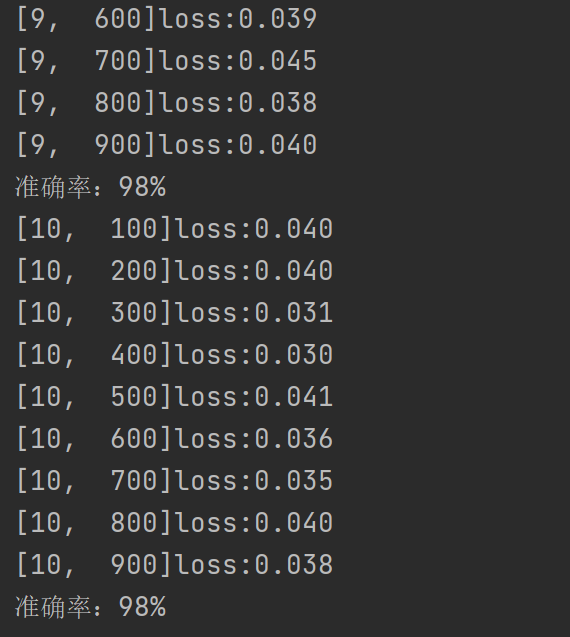
    print('Accuracy:%d%%'%(100*sum_correct/total))

if __name__ == "__main__":
    for epoch in range(10):
        train(epoch)
        test()

If there is a GPU in the device and we want to use the graphics card to speed up the training process, we only need to set whether to use GPU in the code. At this time, all modules of the model and data must be put into CUDA.