1, Pool layer

Pooling operation: to "collect" and "summarize" signals, which is similar to the pool collecting water resources, so it is named pooling layer.

• Collection: from changeable to less, the size of the image changes from large to small
• Summary: maximum / average
  The following is a schematic diagram of maximum pooling and average pooling:
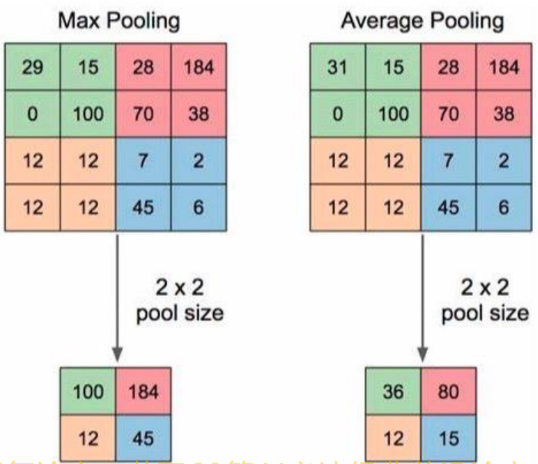  Maximum pooling is to take the maximum value in the sliding window as the final result; Average pooling takes the average value of the sliding window as the final result. Let's take a look at the functions that provide maximum and average pooling in pytorch

1,nn.Maxpool2d

nn.MaxPool2d(kernel_size, stride=None, padding=0, dilation=1, return_indices=False, ceil_mode=False)

Function: pool the maximum value of two-dimensional signal (image)
Parameters:

• kernel_size: pool core size
• Stripe: step size
• Padding: number of padding
• Division: pool core interval size
• ceil_mode: Dimension rounded up
• return_ Indexes: record pooled pixel indexes

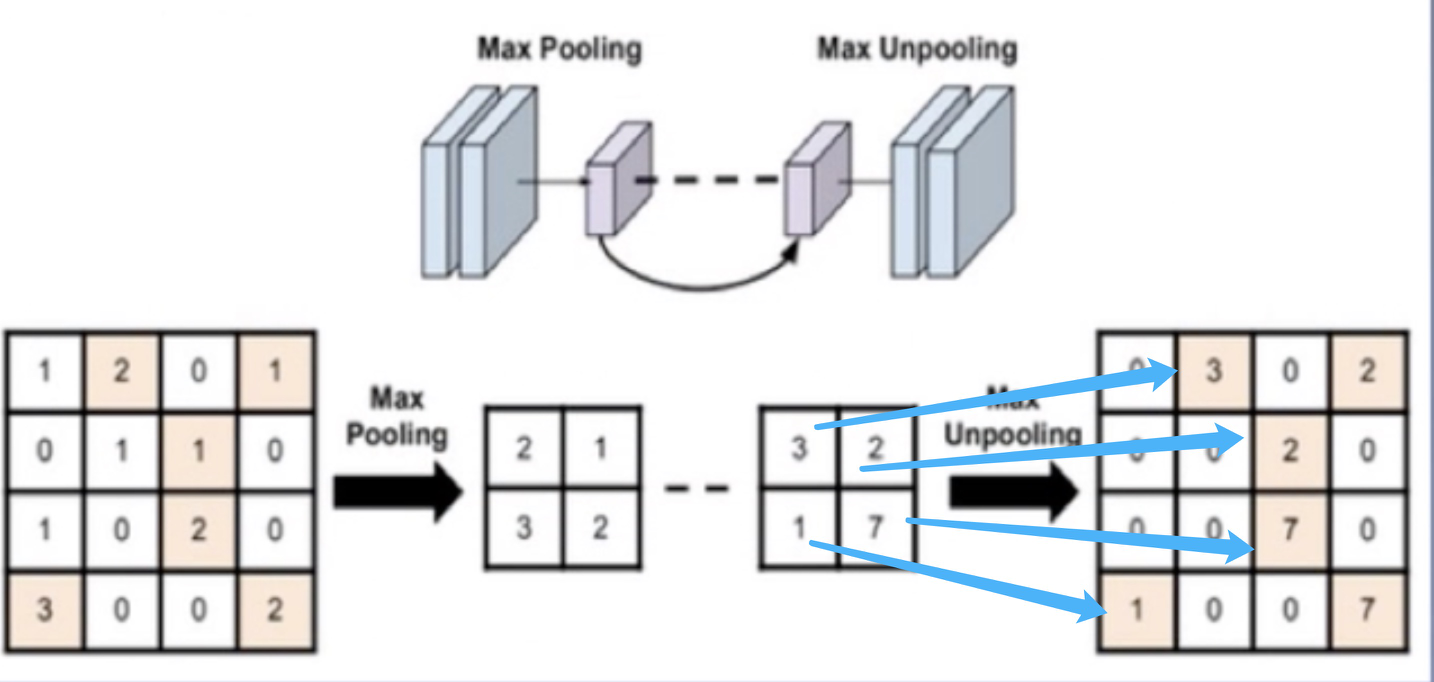
The first several parameters are similar to convolution. The last parameter is often used in maximum anti pooling. It returns the index value of the location of the maximum value in the sliding window. The anti maximum pooling process is shown in the following figure:

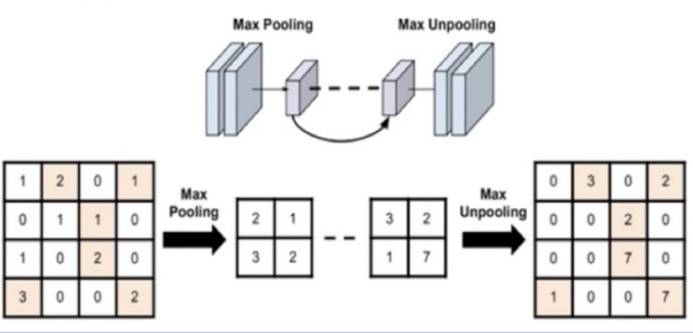
The picture on the left is 4 ✖️ The graph of 4 becomes 2 after pooling the maximum value ✖️ 2. The figure on the right is the anti pooling operation. The smaller figure is changed into a larger figure after up sampling. In the process of anti pooling operation, where should the values in the small figure be placed in the up sampled figure? This requires the index value after the maximum value is pooled. Put the element in the corresponding position according to the index value to get the rightmost image in the figure above.

Let's take a look at the effect of maximum pooling:

# ================================= load img ==================================
path_img = os.path.join(os.path.dirname(os.path.abspath(__file__)), "lena.png")
img = Image.open(path_img).convert('RGB')  # 0~255

# convert to tensor
img_transform = transforms.Compose([transforms.ToTensor()])
img_tensor = img_transform(img)
img_tensor.unsqueeze_(dim=0)    # C*H*W to B*C*H*W

# ================ maxpool
flag = 1
# flag = 0
if flag:
    maxpool_layer = nn.MaxPool2d((2, 2), stride=(2, 2))   # input:(i, o, size) weights:(o, i , h, w)
    img_pool = maxpool_layer(img_tensor)
    
# ================================= visualization ==================================
print("Size before pool:{}\n Size after pool:{}".format(img_tensor.shape, img_pool.shape))
img_pool = transform_invert(img_pool[0, 0:3, ...], img_transform)
img_raw = transform_invert(img_tensor.squeeze(), img_transform)
plt.subplot(122).imshow(img_pool)
plt.subplot(121).imshow(img_raw)
plt.show()

Output result:

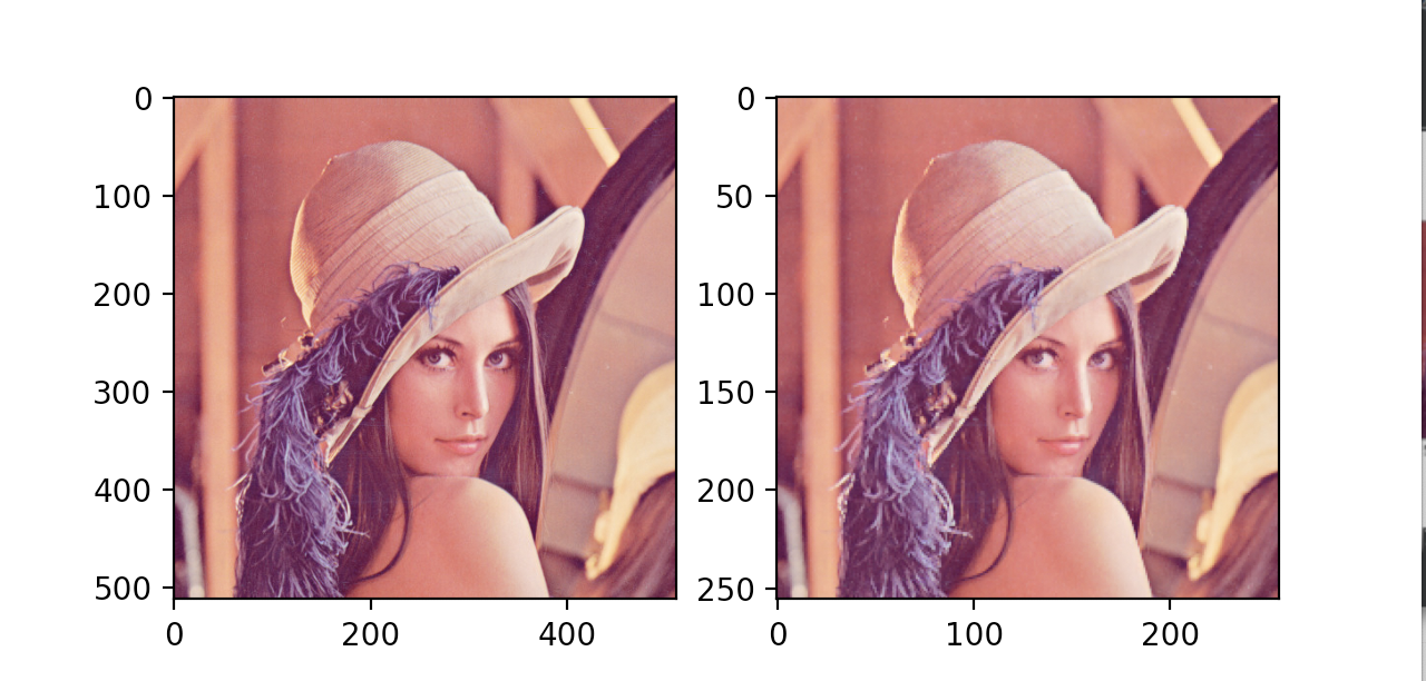
There is basically no difference from the output image, but the size of the image is reduced by half, so the pooling layer can reduce some redundant information in the image.

2,nn.MaxUnpool2d

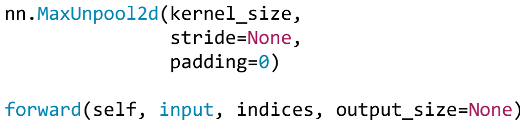
Function: pool up sampling the maximum value of two-dimensional signal (image)
Parameters:
kernel_size: pool core size
Stripe: step size
Padding: number of padding
This parameter is similar to pooling, but it needs to pass in indices during forward propagation. This parameter refers to where the input value is placed in the upper sampling image.

Let's look at the specific implementation process of anti pooling operation through the code:

img_tensor = torch.randint(high=5, size=(1, 1, 4, 4), dtype=torch.float)
maxpool_layer = nn.MaxPool2d((2, 2), stride=(2, 2), return_indices=True)
img_pool, indices = maxpool_layer(img_tensor)

# unpooling
img_reconstruct = torch.randn_like(img_pool, dtype=torch.float)
maxunpool_layer = nn.MaxUnpool2d((2, 2), stride=(2, 2))
img_unpool = maxunpool_layer(img_reconstruct, indices)

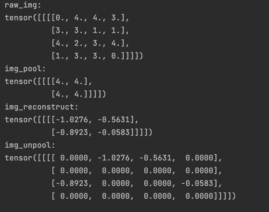
print("raw_img:\n{}\nimg_pool:\n{}".format(img_tensor, img_pool))
print("img_reconstruct:\n{}\nimg_unpool:\n{}".format(img_reconstruct, img_unpool))

Output result:

3,nn.AvgPool2d

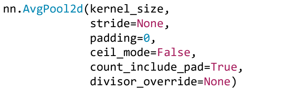
Function: pool the average value of two-dimensional signals (images)
Parameters:
count_include_pad: the filling value is used for calculation
divisor_override: division factor. This parameter is the denominator when averaging. By default, several numbers are added and divided by several. It can also be set through this parameter

Specific implementation process:

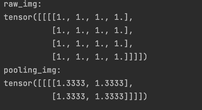
img_tensor = torch.ones((1, 1, 4, 4))
avgpool_layer = nn.AvgPool2d((2, 2), stride=(2, 2), divisor_override=3)   #When averaging, the denominator is 3
img_pool = avgpool_layer(img_tensor)

print("raw_img:\n{}\npooling_img:\n{}".format(img_tensor, img_pool))

Output result:

2, Linear layer

The linear layer is also called the full connection layer. Each neuron is connected with all neurons of the previous layer to realize the linear combination and linear transformation of the previous layer.
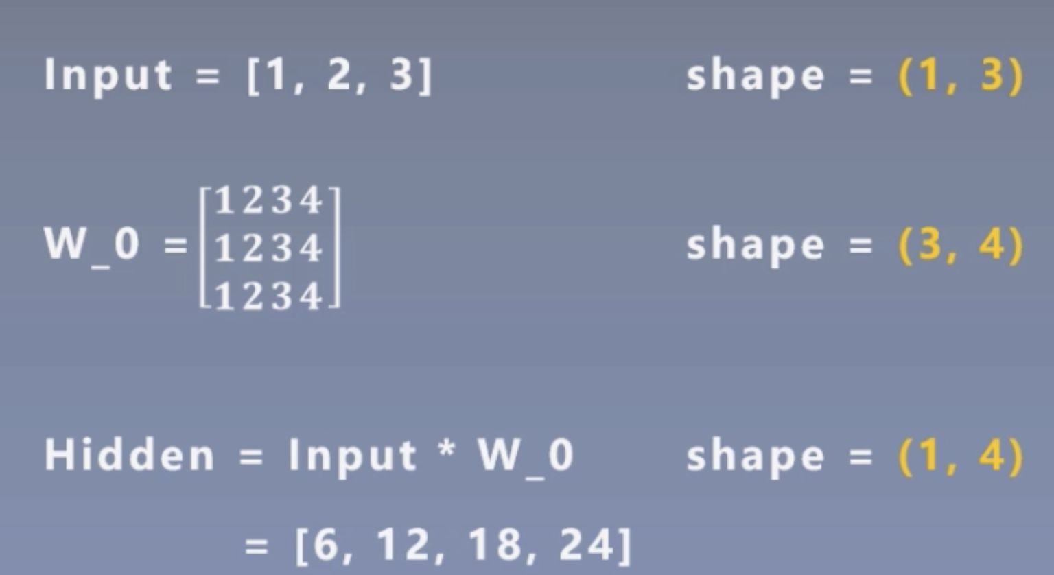
The linear calculation of the layer is shown in the figure below:

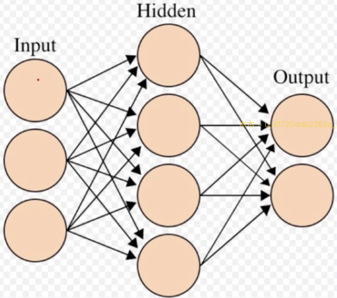
The input of each layer is obtained by multiplying and adding the neurons of the previous layer. The calculation process is as follows:

Implementation of code in pytorch

nn.Linear(in_features, out_features, bias=True)

Function: linear combination of one-dimensional vectors (signals)
Parameters:

• in_features: enter the number of nodes
• out_features: number of output nodes
• bias: whether offset is required. The default value is True
  Calculation formula:
  

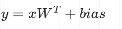
inputs = torch.tensor([[1., 2, 3]])
linear_layer = nn.Linear(3, 4)
# Initialization of weights
linear_layer.weight.data = torch.tensor([[1., 1., 1.],
                                         [2., 2., 2.],
                                         [3., 3., 3.],
                                         [4., 4., 4.]])
#Initialization value of offset
linear_layer.bias.data.fill_(0.5)
output = linear_layer(inputs)
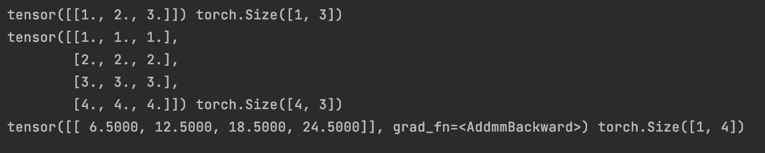
print(inputs, inputs.shape)
print(linear_layer.weight.data, linear_layer.weight.data.shape)
print(output, output.shape)

Output result: