Multilayer perceptron

Both linear regression and softmax regression are single-layer neural networks. However, deep learning mainly focuses on multi-layer models. Taking multilayer perceptron (MLP) as an example, the concept of multilayer neural network is introduced.

Hidden layer

Multilayer perceptron introduces one or more hidden layers based on single-layer neural network. The hidden layer is between the input layer and the output layer. The figure shows the neural network diagram of a multi-layer perceptron, which contains a hidden layer with five hidden units.

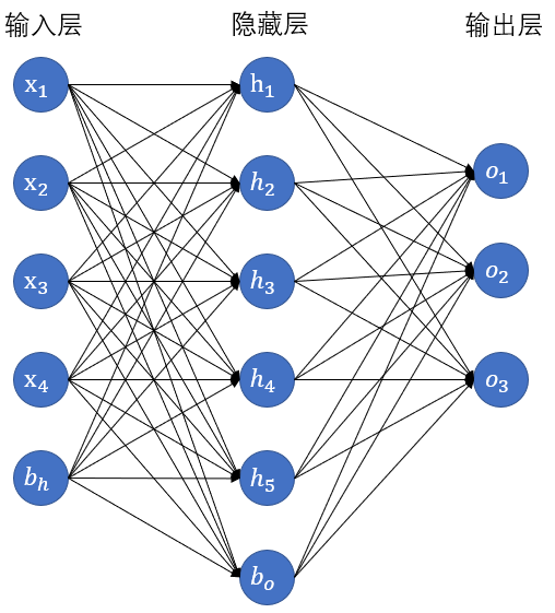
In the multi-layer perceptron shown in the figure, the number of inputs and outputs are 4 and 3 respectively, and the middle hidden layer contains five hidden unit s. Since the input layer does not involve calculation, the number of layers of the multi-layer perceptron in Figure 3.3 is 2. As can be seen from the figure, the neurons in the hidden layer are fully connected with each input in the input layer, and the neurons in the output layer are also fully connected with each neuron in the hidden layer. Therefore, the hidden layer and output layer in the multi-layer perceptron are all connected layers.

Specifically, given a small batch of samples X ∈ R n × d \boldsymbol{X} \in \mathbb{R}^{n \times d} X∈Rn × d. Its batch size is n n n. The number of entries is d d d. Suppose that the multi-layer perceptron has only one hidden layer, in which the number of hidden units is h h h. Note that the output of the hidden layer (also known as hidden layer variable or hidden variable) is H \boldsymbol{H} H. Yes H ∈ R n × h \boldsymbol{H} \in \mathbb{R}^{n \times h} H∈Rn × h. Because the hidden layer and the output layer are all connected layers, the weight parameters and deviation parameters of the hidden layer can be set as W h ∈ R d × h \boldsymbol{W}_h \in \mathbb{R}^{d \times h} Wh​∈Rd × h and b h ∈ R 1 × h \boldsymbol{b}_h \in \mathbb{R}^{1 \times h} bh​∈R1 × h. The weight and deviation parameters of the output layer are W o ∈ R h × q \boldsymbol{W}_o \in \mathbb{R}^{h \times q} Wo​∈Rh × q and b o ∈ R 1 × q \boldsymbol{b}_o \in \mathbb{R}^{1 \times q} bo​∈R1×q.

Let's first look at the design of a multi-layer perceptron with a single hidden layer. Its output O ∈ R n × q \boldsymbol{O} \in \mathbb{R}^{n \times q} O∈Rn × The calculation of q is

H = X W h + b h , O = H W o + b o , \begin{aligned} \boldsymbol{H} &= \boldsymbol{X} \boldsymbol{W}_h + \boldsymbol{b}_h,\\ \boldsymbol{O} &= \boldsymbol{H} \boldsymbol{W}_o + \boldsymbol{b}_o, \end{aligned} HO​=XWh​+bh​,=HWo​+bo​,​

That is, the output of the hidden layer is directly used as the input of the output layer. If the above two equations are combined, we can get

O = ( X W h + b h ) W o + b o = X W h W o + b h W o + b o . \boldsymbol{O} = (\boldsymbol{X} \boldsymbol{W}_h + \boldsymbol{b}_h)\boldsymbol{W}_o + \boldsymbol{b}_o = \boldsymbol{X} \boldsymbol{W}_h\boldsymbol{W}_o + \boldsymbol{b}_h \boldsymbol{W}_o + \boldsymbol{b}_o. O=(XWh​+bh​)Wo​+bo​=XWh​Wo​+bh​Wo​+bo​.

It can be seen from the simultaneous formula that although the neural network introduces a hidden layer, it is still equivalent to a single-layer neural network: the weight parameter of the output layer is W h W o \boldsymbol{W}_h\boldsymbol{W}_o Wh Wo, deviation parameter is b h W o + b o \boldsymbol{b}_h \boldsymbol{W}_o + \boldsymbol{b}_o bh​Wo​+bo​. It is not difficult to find that even if more hidden layers are added, the above design can only be equivalent to the single-layer neural network with only output layer.

Activation function

The root of the above problem is that the full connection layer only makes affine transformation on the data, and the superposition of multiple affine transformations is still an affine transformation. One way to solve the problem is to introduce nonlinear transformation. For example, the hidden variables are transformed by using the nonlinear function operated by elements, and then used as the input of the next full connection layer. This nonlinear function is called activation function. Let's introduce some common activation functions.

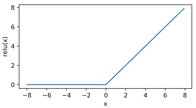
The ReLU (rectified linear unit) function provides a very simple nonlinear transformation. Given element x x x. This function is defined as

ReLU ( x ) = max ⁡ ( x , 0 ) . \text{ReLU}(x) = \max(x, 0). ReLU(x)=max(x,0).

It can be seen that the ReLU function only retains positive elements and clears negative elements. In order to observe this nonlinear transformation intuitively, we first define a drawing function xyplot.

%matplotlib inline
import torch
import numpy as np
import matplotlib.pylab as plt
from IPython import display

def use_svg_display():
    """"use svg Format display graphics"""
    display.set_matplotlib_formats('svg')

def set_figsize(figsize=(3.5, 2.5)):
    use_svg_display()
    # Set the size of the drawing
    plt.rcParams['figure.figsize'] = figsize

def xyplot(x_vals, y_vals, name):
    set_figsize(figsize=(5, 2.5))
    plt.plot(x_vals.detach().numpy(), y_vals.detach().numpy())
    plt.xlabel('x')
    plt.ylabel(name + '(x)')

Draw the relu function through the relu function provided by Tensor. It can be seen that the activation function is a two segment linear function.

x = torch.arange(-8.0, 8.0, 0.1, requires_grad=True)
y = x.relu()
xyplot(x, y, 'relu')

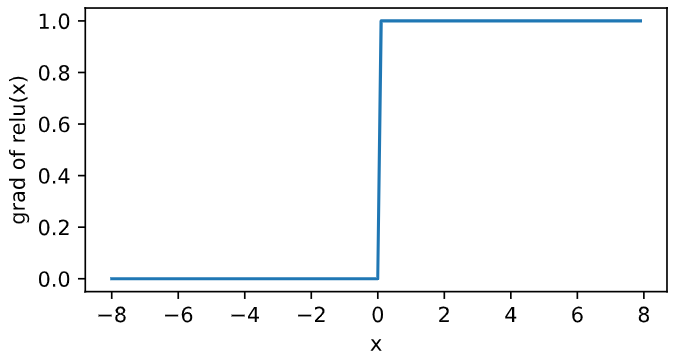
Obviously, when the input is negative, the derivative of ReLU function is 0; When the input is positive, the derivative of the ReLU function is 1. Although the ReLU function is not differentiable when the input is 0, we can take the derivative here as 0. The derivative of the ReLU function is plotted below.

y.sum().backward()
xyplot(x, x.grad, 'grad of relu')

sigmoid function

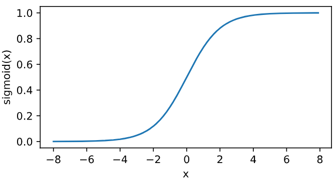
The sigmoid function can transform the value of an element between 0 and 1:

sigmoid ( x ) = 1 1 + exp ⁡ ( − x ) . \text{sigmoid}(x) = \frac{1}{1 + \exp(-x)}. sigmoid(x)=1+exp(−x)1​.

Sigmoid function is common in early neural networks, but it is gradually replaced by simpler ReLU function. However, it can use its value range between 0 and 1 to control the flow of information in neural network, which will not be discussed here. The sigmoid function is drawn below. When the input is close to 0, the sigmoid function is close to the linear transformation.

y = x.sigmoid()
xyplot(x, y, 'sigmoid')

According to the chain rule, the derivative of sigmoid function

sigmoid ′ ( x ) = sigmoid ( x ) ( 1 − sigmoid ( x ) ) . \text{sigmoid}'(x) = \text{sigmoid}(x)\left(1-\text{sigmoid}(x)\right). sigmoid′(x)=sigmoid(x)(1−sigmoid(x)).

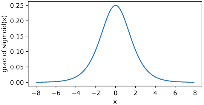
The derivative of sigmoid function is plotted below. When the input is 0, the derivative of sigmoid function reaches the maximum value of 0.25; When the input deviates from 0, the derivative of sigmoid function approaches 0.

x.grad.zero_()
y.sum().backward()
xyplot(x, x.grad, 'grad of sigmoid')

tanh function

The tanh (hyperbolic tangent) function transforms the value of an element between - 1 and 1:

tanh ( x ) = 1 − exp ⁡ ( − 2 x ) 1 + exp ⁡ ( − 2 x ) . \text{tanh}(x) = \frac{1 - \exp(-2x)}{1 + \exp(-2x)}. tanh(x)=1+exp(−2x)1−exp(−2x)​.

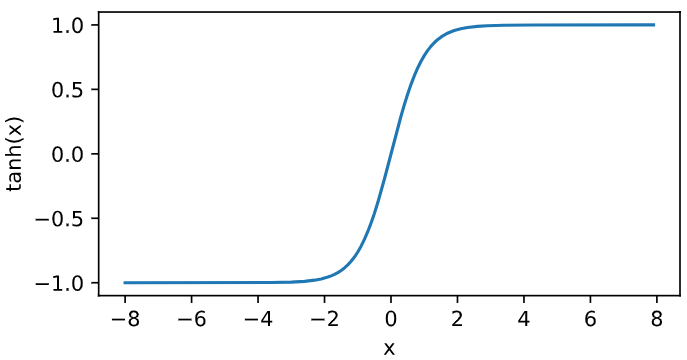
We then plot the tanh function. When the input is close to 0, the tanh function is close to the linear transformation. Although the shape of the function is very similar to that of sigmoid function, the tanh function is symmetrical at the origin of the coordinate system.

y = x.tanh()
xyplot(x, y, 'tanh')

According to the chain rule, the derivative of tanh function

tanh ′ ( x ) = 1 − tanh 2 ( x ) . \text{tanh}'(x) = 1 - \text{tanh}^2(x). tanh′(x)=1−tanh2(x).

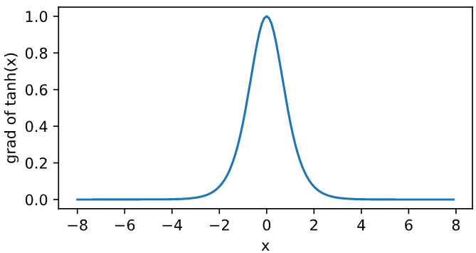
The derivative of the tanh function is plotted below. When the input is 0, the derivative of tanh function reaches the maximum value of 1; When the input deviates from 0, the derivative of tanh function approaches 0.

x.grad.zero_()
y.sum().backward()
xyplot(x, x.grad, 'grad of tanh')

Multilayer perceptron

Multilayer perceptron is a neural network composed of fully connected layers with at least one hidden layer, and the output of each hidden layer is transformed by activation function. The number of layers of multi-layer perceptron and the number of hidden units in each hidden layer are super parameters. Taking a single hidden layer as an example, the multi-layer perceptron calculates the output in the following way:

H = ϕ ( X W h + b h ) , O = H W o + b o , \begin{aligned} \boldsymbol{H} &= \phi(\boldsymbol{X} \boldsymbol{W}_h + \boldsymbol{b}_h),\\ \boldsymbol{O} &= \boldsymbol{H} \boldsymbol{W}_o + \boldsymbol{b}_o, \end{aligned} HO​=ϕ(XWh​+bh​),=HWo​+bo​,​

among ϕ \phi ϕ Indicates the activation function. In the classification problem, we can analyze the output O \boldsymbol{O} O do softmax operation and use the cross entropy loss function in softmax regression.
In the regression problem, we set the number of outputs of the output layer to 1 and O \boldsymbol{O} O is directly provided to the square loss function used in linear regression.

Summary

• The multi-layer perceptron adds one or more fully connected hidden layers between the output layer and the input layer, and transforms the output of the hidden layer through the activation function.
• Common activation functions include ReLU function, sigmoid function and tanh function.

PyTorch realizes multi-layer perceptron from scratch

We have understood the principle of multilayer perceptron. First, import the package or module required for implementation.

import torch
import numpy as np
import sys
import torchvision

Get and read data

The fashion MNIST dataset continues to be used here. We will use multi-layer perceptron to classify images.

def load_data_fashion_mnist(batch_size, resize=None, root='~/Datasets/FashionMNIST'):
    """: download fashion mnist The dataset is then loaded into memory."""
    trans = []
    if resize:
        trans.append(torchvision.transforms.Resize(size=resize))
    trans.append(torchvision.transforms.ToTensor())
    
    transform = torchvision.transforms.Compose(trans)
    mnist_train = torchvision.datasets.FashionMNIST(root=root, train=True, download=True, transform=transform)
    mnist_test = torchvision.datasets.FashionMNIST(root=root, train=False, download=True, transform=transform)
    if sys.platform.startswith('win'):
        num_workers = 0  # 0 means no additional process is needed to speed up the reading of data
    else:
        num_workers = 4
    train_iter = torch.utils.data.DataLoader(mnist_train, batch_size=batch_size, shuffle=True, num_workers=num_workers)
    test_iter = torch.utils.data.DataLoader(mnist_test, batch_size=batch_size, shuffle=False, num_workers=num_workers)

    return train_iter, test_iter

batch_size = 256
train_iter, test_iter = load_data_fashion_mnist(batch_size)

Define model parameters

The image shape in the fashion MNIST dataset is 28 × 28 28 \times 28 twenty-eight × 28. The number of categories is 10. We still use a length of 28 × 28 = 784 28 \times 28 = 784 twenty-eight × A vector of 28 = 784 represents each image. Therefore, the number of inputs is 784 and the number of outputs is 10. In the experiment, we set the number of hyperparametric hiding units to 256.

num_inputs, num_outputs, num_hiddens = 784, 10, 256

W1 = torch.tensor(np.random.normal(0, 0.01, (num_inputs, num_hiddens)), dtype=torch.float)
b1 = torch.zeros(num_hiddens, dtype=torch.float)
W2 = torch.tensor(np.random.normal(0, 0.01, (num_hiddens, num_outputs)), dtype=torch.float)
b2 = torch.zeros(num_outputs, dtype=torch.float)

params = [W1, b1, W2, b2]
for param in params:
    param.requires_grad_(requires_grad=True)

Define activation function

Here, we use the basic max function to implement relu instead of calling the relu function directly.

def relu(X):
    return torch.max(input=X, other=torch.tensor(0.0))

Define model

Like softmax regression, we change the length of each original image to num through the view function_ Vector of inputs. Then we implement the computational expression of multilayer perceptron.

def net(X):
    X = X.view((-1, num_inputs))
    H = relu(torch.matmul(X, W1) + b1)
    return torch.matmul(H, W2) + b2

Define loss function

In order to obtain better numerical stability, we directly use the functions provided by PyTorch, including softmax operation and cross entropy loss calculation.

loss = torch.nn.CrossEntropyLoss()

Training model

There is no difference between the steps of training multilayer perceptron and the steps of training softmax regression. Here, we set the number of hyperparametric iteration cycles to 5 and the learning rate to 100.0.

Note: since SoftmaxCrossEntropyLoss in mxnet of hands-on deep learning is summed along the batch dimension during back propagation, and PyTorch is averaged by default, the loss calculated by PyTorch is much smaller than that of mxnet (about the order of 1/batch_size calculated by maxnet), so the gradient obtained by back propagation is also much smaller, So in order to get the same learning effect, we adjusted the learning rate to about batch of the original book_ Size times, the learning rate of the original book is 0.5, which is set to 100.0 here. (the reason why it is so large is that the sgd function is divided by batch_size when updating. In fact, PyTorch has been divided once when calculating loss. sgd should not be divided here.)

def sgd(params, lr, batch_size):
    # In order to be consistent with "hands-on learning and deep learning", this is divided by batch_size, but it should not be divided, because PyTorch is usually used to calculate loss by default
    # Average along the batch dimension.
    for param in params:
        param.data -= lr * param.grad / batch_size # Note the param. Used when changing param here data
        
def evaluate_accuracy(data_iter, net):
    acc_sum, n = 0.0, 0
    for X, y in data_iter:
        acc_sum += (net(X).argmax(dim=1) == y).float().sum().item()
        n += y.shape[0]
    return acc_sum / n

def train(net, train_iter, test_iter, loss, num_epochs, batch_size,
              params=None, lr=None, optimizer=None):
    for epoch in range(num_epochs):
        train_l_sum, train_acc_sum, n = 0.0, 0.0, 0
        for X, y in train_iter:
            y_hat = net(X)
            l = loss(y_hat, y).sum()
            
            # Gradient clearing
            if optimizer is not None:
                optimizer.zero_grad()
            elif params is not None and params[0].grad is not None:
                for param in params:
                    param.grad.data.zero_()
            
            l.backward()
            if optimizer is None:
                sgd(params, lr, batch_size)
            else:
                optimizer.step()  
            
            
            train_l_sum += l.item()
            train_acc_sum += (y_hat.argmax(dim=1) == y).sum().item()
            n += y.shape[0]
        test_acc = evaluate_accuracy(test_iter, net)
        print('epoch %d, loss %.4f, train acc %.3f, test acc %.3f'
              % (epoch + 1, train_l_sum / n, train_acc_sum / n, test_acc))
num_epochs, lr = 5, 100.0
train(net, train_iter, test_iter, loss, num_epochs, batch_size, params, lr)

epoch 1, loss 0.0031, train acc 0.711, test acc 0.745
epoch 2, loss 0.0019, train acc 0.824, test acc 0.780
epoch 3, loss 0.0017, train acc 0.845, test acc 0.785
epoch 4, loss 0.0015, train acc 0.855, test acc 0.854
epoch 5, loss 0.0015, train acc 0.864, test acc 0.830

Summary

• A simple multi-layer perceptron can be realized by manually defining the model and its parameters, but it is limited to helping understand its principle logic. In the actual process, it is generally realized by using the framework module.
• When there are many layers of multi-layer perceptron, the implementation method from zero will be more cumbersome, such as when defining model parameters.

PyTorch module realizes multi-layer perceptron

Next, we use PyTorch module to implement multi-layer perceptron. First import the required package or module.

import torch
from torch import nn
from torch.nn import init
import numpy as np
import sys

Define model

The only difference from softmax regression is that we add a full connection layer as the hidden layer. It has 256 hidden units and uses the ReLU function as the activation function.

num_inputs, num_outputs, num_hiddens = 784, 10, 256

class FlattenLayer(torch.nn.Module): # Full connection layer
    def __init__(self):
        super(FlattenLayer, self).__init__()
    def forward(self, x): # x shape: (batch, *, *, ...)
        return x.view(x.shape[0], -1)

net = nn.Sequential(
        FlattenLayer(),
        nn.Linear(num_inputs, num_hiddens),
        nn.ReLU(),
        nn.Linear(num_hiddens, num_outputs), 
        )

for params in net.parameters():
    init.normal_(params, mean=0, std=0.01)

Read data and train model

We use almost the same steps as training softmax regression to read the data and train the model.

Note: the SGD of PyTorch is used here

batch_size = 256
def load_data_fashion_mnist(batch_size, resize=None, root='~/Datasets/FashionMNIST'):
    """: download fashion mnist The dataset is then loaded into memory."""
    trans = []
    if resize:
        trans.append(torchvision.transforms.Resize(size=resize))
    trans.append(torchvision.transforms.ToTensor())
    
    transform = torchvision.transforms.Compose(trans)
    mnist_train = torchvision.datasets.FashionMNIST(root=root, train=True, download=True, transform=transform)
    mnist_test = torchvision.datasets.FashionMNIST(root=root, train=False, download=True, transform=transform)
    if sys.platform.startswith('win'):
        num_workers = 0  # 0 means no additional process is needed to speed up the reading of data
    else:
        num_workers = 4
    train_iter = torch.utils.data.DataLoader(mnist_train, batch_size=batch_size, shuffle=True, num_workers=num_workers)
    test_iter = torch.utils.data.DataLoader(mnist_test, batch_size=batch_size, shuffle=False, num_workers=num_workers)

    return train_iter, test_iter
train_iter, test_iter = load_data_fashion_mnist(batch_size)
loss = torch.nn.CrossEntropyLoss()

optimizer = torch.optim.SGD(net.parameters(), lr=0.5)

num_epochs = 5

def train(net, train_iter, test_iter, loss, num_epochs, batch_size,
              params=None, lr=None, optimizer=None):
    for epoch in range(num_epochs):
        train_l_sum, train_acc_sum, n = 0.0, 0.0, 0
        for X, y in train_iter:
            y_hat = net(X)
            l = loss(y_hat, y).sum()
            
            # Gradient clearing
            if optimizer is not None:
                optimizer.zero_grad()
            elif params is not None and params[0].grad is not None:
                for param in params:
                    param.grad.data.zero_()
            
            l.backward()
            if optimizer is None:
                sgd(params, lr, batch_size)
            else:
                optimizer.step() 
            
            
            train_l_sum += l.item()
            train_acc_sum += (y_hat.argmax(dim=1) == y).sum().item()
            n += y.shape[0]
        test_acc = evaluate_accuracy(test_iter, net)
        print('epoch %d, loss %.4f, train acc %.3f, test acc %.3f'
              % (epoch + 1, train_l_sum / n, train_acc_sum / n, test_acc))

train(net, train_iter, test_iter, loss, num_epochs, batch_size, None, None, optimizer)

epoch 1, loss 0.0032, train acc 0.692, test acc 0.771
epoch 2, loss 0.0019, train acc 0.814, test acc 0.800
epoch 3, loss 0.0016, train acc 0.846, test acc 0.803
epoch 4, loss 0.0015, train acc 0.856, test acc 0.823
epoch 5, loss 0.0015, train acc 0.862, test acc 0.848

Summary

• The multi-layer perceptron can be realized more concisely through PyTorch module.

reference resources

[1] Aston Zhang, Mu Li, Zachary C.Lipton, etc Hands on learning and deep learning Beijing: People's Posts and Telecommunications Press, 2019

[2] https://pytorch.org/docs/stable/index.html

[3] https://github.com/ShusenTang/Dive-into-DL-PyTorch