I Introduction to ResNet algorithm

Residual neural network (ResNet) was proposed by he Kaiming of Microsoft Research Institute. ResNet won the championship in ILSVRC in 2015.

Through experiments, ResNet has continuously improved the accuracy of the model with the deepening of the network layer, Reach the maximum (accuracy saturation), and then with the continuous increase of network depth, the accuracy of the model decreases significantly without warning. This phenomenon is obviously contradictory and conflicting with the belief that "the deeper the network, the higher the accuracy". ResNet team calls this phenomenon "Degradation".

It is reasonable to add more layers to the network. The solution space of the shallow network is contained in the solution space of the deep network. The solution space of the deep network is at least no worse than that of the shallow network, because you can obtain the same performance as the shallow network by simply turning the added layer into an identity map and keeping the weight of other layers intact. A better solution clearly exists, why can't it be found? Found a worse solution instead?

The performance degradation on the training set can eliminate over fitting, and the introduction of BN layer basically solves the problems of gradient disappearance and gradient explosion. If it is not caused by over fitting and gradient disappearance, what is the reason?

Obviously, this is an optimization problem, which reflects that the optimization difficulty of models with similar structure is different, and the increase of difficulty is not linear. The deeper the model, the more difficult it is to optimize.

There are two solutions. One is to adjust the solution method, such as better initialization, better gradient descent algorithm, etc; The other is to adjust the model structure to make the model easier to optimize - changing the model structure actually changes the shape of the error surface.

ResNet puts forward the concept of residual block from the perspective of adjusting the model structure. The practical principle is to let each residual block in the deep layer of the network learn identities as much as possible. This is equivalent to simplifying the task, and the network depth can be deeper.

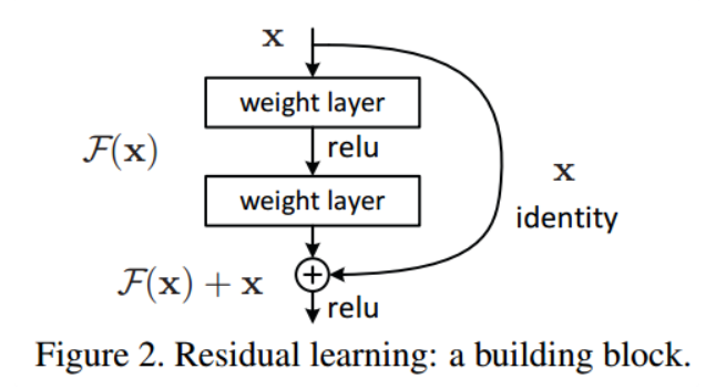
Why is the residual block designed like this?

The purpose of ResNet is to design an identity mapping network, but the task of fitting identity by neural network is more complex, so it is better to directly learn the mapping of residuals. Then the purpose of the network is to make the residual equal to zero, which is equivalent to an identity mapping network. As shown in Figure 2, it is a residual block, F(x) represents the residual learning path, X represents the shortcut path, and the mapping relationship obtained after learning is:

In the original paper, the residual paths can be roughly divided into two types. One has a bottleneck structure, that is, 1 in the right of the figure below × 1. Convolution layer is used to reduce the dimension first and then increase the dimension. It is mainly for the practical consideration of reducing the computational complexity. It is called "bottleneck block". The other without bottleneck structure is called "basic block", as shown on the left of the figure below. Basic block consists of 2 3 × 3. Composition of convolution layer.

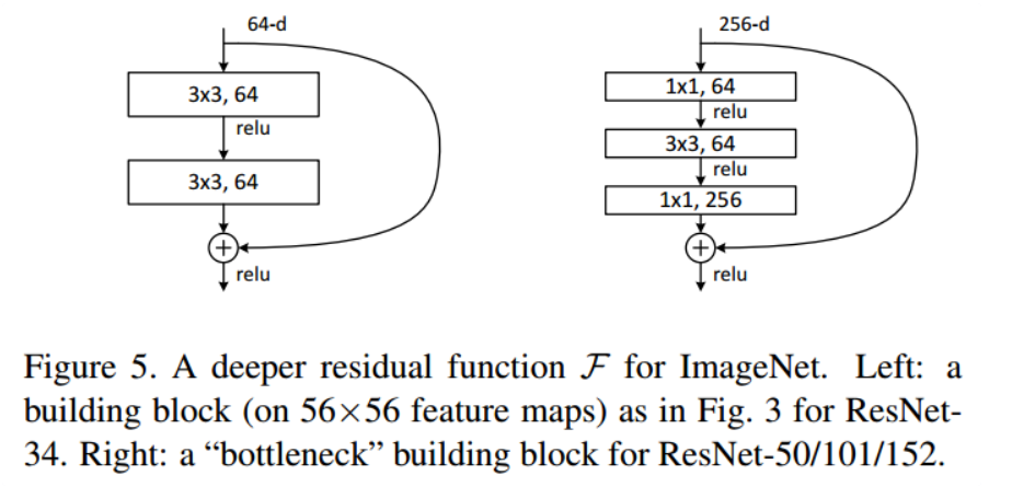
ResNet is a series of multiple residual blocks. Its structure is very easy to modify and expand. By adjusting the number of channel s in the block and the number of stacked blocks, it is easy to adjust the width and depth of the network to obtain networks with different expression abilities without worrying too much about the "degradation" of the network. As long as the training data is sufficient, the network can be deepened step by step, You can get better performance. At present, ResNet is most often used as the backbone of the detection network. The commonly used structures include ResNet-50, ResNet-101, etc.

2, Data set introduction

This experiment uses the open source data set of gesture recognition to train a gesture classifier. Data set from project https://codechina.csdn.net/EricLee/classification , a total of 2850 samples were divided into 14 categories.

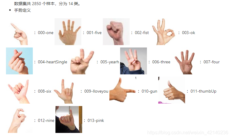
There is nothing to say about the pytorch definition of data. The basic steps are as follows. You can rewrite several functions according to your own data characteristics. In this experiment, the samples are divided into training set and verification set according to the ratio of 5:1.

import torch
import torch.nn as nn
from torch.utils.data import DataLoader,Dataset
from torchvision import transforms as T
import matplotlib.pyplot as plt
import os
from PIL import Image
import numpy as np
import random
 
class hand_pose(Dataset):
    def __init__(self, root, train=True, transforms=None):
        imgs = []
        for path in os.listdir(root):
            path_prefix = path[:3]
            if path_prefix == "000":
                label = 0
            elif path_prefix == "001":
                label = 1
            elif path_prefix == "002":
                label = 2
            elif path_prefix == "003":
                label = 3
            elif path_prefix == "004":
                label = 4
            elif path_prefix == "005":
                label = 5
            elif path_prefix == "006":
                label = 6
            elif path_prefix == "007":
                label = 7
            elif path_prefix == "008":
                label = 8
            elif path_prefix == "009":
                label = 9
            elif path_prefix == "010":
                label = 10
            elif path_prefix == "011":
                label = 11
            elif path_prefix == "012":
                label = 12
            elif path_prefix == "013":
                label = 13
            else:
                print("data label error")
 
            childpath = os.path.join(root, path)
            for imgpath in os.listdir(childpath):
                imgs.append((os.path.join(childpath, imgpath), label))
        
        train_path_list, val_path_list = self._split_data_set(imgs)
        if train:
            self.imgs = train_path_list
        else:
            self.imgs = val_path_list

        if transforms is None:
            normalize = T.Normalize(mean=[0.485, 0.456, 0.406], std=[0.229, 0.224, 0.225])
 
            self.transforms = T.Compose([
                    T.Resize(256),
                    T.CenterCrop(224),
                    T.ToTensor(),
                    normalize
            ])
        else:
            self.transforms = transforms
             
    def __getitem__(self, index):
        img_path = self.imgs[index][0]
        label = self.imgs[index][1]
 
        data = Image.open(img_path)
        if data.mode != "RGB":
            data = data.convert("RGB")
        data = self.transforms(data)
        return data,label
 
    def __len__(self):
        return len(self.imgs)

    def _split_data_set(self, imags):
        """
        The classified data are training set and verification set, which are designed according to the characteristics of personal data and are not universal.
        """
        val_path_list = imags[::5]
        train_path_list = []
        for item in imags:
            if item not in val_path_list:
                train_path_list.append(item)
        return train_path_list, val_path_list
 
if __name__ == "__main__":
    root = "handpose_x_gesture_v1"
   
    train_dataset = hand_pose(root, train=False)
    train_dataloader = DataLoader(train_dataset, batch_size=32, shuffle=True)
    for data, label in train_dataloader:
        print(data.shape)
        print(label)
        break

Because NN Crossentroyloss contains softmax and ont hot encoding processing, so there is no need to perform ont hot processing during data definition, and the categories can be sorted according to int (0, 1, 2

Three, model training

3.1 model network definition

import torch
from torch import nn

class Bottleneck(nn.Module):
    # Residual block definition
    extention = 4
    def __init__(self, inplanes, planes, stride, downsample=None):
        super(Bottleneck, self).__init__()
        self.conv1 = nn.Conv2d(inplanes, planes, kernel_size=1, stride=stride, bias=False)
        self.bn1 = nn.BatchNorm2d(planes)

        self.conv2 = nn.Conv2d(planes, planes, kernel_size=3, stride=1, padding=1, bias=False)
        self.bn2 = nn.BatchNorm2d(planes)

        self.conv3 = nn.Conv2d(planes, planes*self.extention, kernel_size=1, stride=1, bias=False)
        self.bn3 = nn.BatchNorm2d(planes*self.extention)

        self.relu = nn.ReLU(inplace=True)

        self.downsample = downsample
        self.stride = stride

    def forward(self, x):
        shortcut = x

        out = self.conv1(x)
        out = self.bn1(out)
        out = self.relu(out)

        out = self.conv2(out)
        out = self.bn2(out)
        out = self.relu(out)

        out = self.conv3(out)
        out = self.bn3(out)
        out = self.relu(out)

        if self.downsample is not None:
            shortcut = self.downsample(x)
        
        out = out + shortcut   # Cannot write out+=shortcut
        out = self.relu(out)
        return out


class ResNet50(nn.Module):
    def __init__(self, block, layers, num_class):
        self.inplane = 64
        super(ResNet50,self).__init__()

        self.block = block
        self.layers = layers

        self.conv1 = nn.Conv2d(3, self.inplane, kernel_size=7, stride=2, padding=3, bias=False)
        self.bn1 = nn.BatchNorm2d(self.inplane)
        self.relu = nn.ReLU()
        self.maxpool = nn.MaxPool2d(kernel_size=3, stride=2, padding=1)

        self.stage1=self.make_layer(self.block,64,layers[0],stride=1)
        self.stage2=self.make_layer(self.block,128,layers[1],stride=2)
        self.stage3=self.make_layer(self.block,256,layers[2],stride=2)
        self.stage4=self.make_layer(self.block,512,layers[3],stride=2)

        self.avgpool = nn.AvgPool2d(7)
        self.fc = nn.Linear(512*block.extention, num_class)

    def forward(self, x):
        out = self.conv1(x)
        out = self.bn1(out)
        out = self.relu(out)
        out = self.maxpool(out)

        #block part
        out=self.stage1(out)
        out=self.stage2(out)
        out=self.stage3(out)
        out=self.stage4(out)

        out=self.avgpool(out)
        out=torch.flatten(out,1)
        out=self.fc(out)

        return out

    def make_layer(self, block, plane, block_num, stride=1):
        block_list = []
        downsample = None
        if(stride!=1 or self.inplane!=plane*block.extention):
            downsample = nn.Sequential(
                nn.Conv2d(self.inplane, plane*block.extention, stride=stride, kernel_size=1, bias=False),
                nn.BatchNorm2d(plane*block.extention)
            )
        conv_block = block(self.inplane, plane, stride=stride, downsample=downsample)
        block_list.append(conv_block)
        self.inplane = plane*block.extention

        for i in range(1,block_num):
            block_list.append(block(self.inplane, plane, stride=1))

        return nn.Sequential(*block_list)


if __name__ == "__main__":
    resnet = ResNet50(Bottleneck,[3,4,6,3],14)
    x = torch.randn(64,3,224,224)
    x = resnet(x)
    print(x.shape)

There are two parts of network definition. bottleneck is the basic module of residual network, and Resnet50 is the whole network architecture, which corresponds to the network structure in the figure below.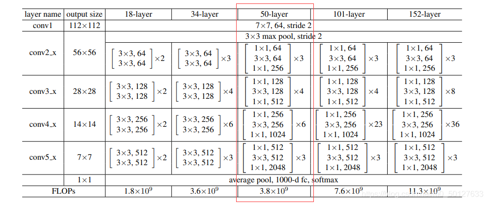  

Note that when defining the residual block bottleneck, the jump and join addition part of the shortcut cannot be written as out += shortcut. The specific reason is that out needs to be saved for the gradient calculation of the back end, and + = is the inplace operation, which changes the variable.

If you write in place, an error will be reported. The error information is:

RuntimeError: one of the variables needed for gradient computation has been modified by an inplace operation:

3.2 training

import torch
import torch.nn as nn
from torch.utils.data import DataLoader,Dataset
from Data import hand_pose
from Model import ResNet50, Bottleneck
import os


def main():
    # 1. load dataset
    root = "handpose_x_gesture_v1"
    batch_size = 64
    train_data = hand_pose(root, train=True)
    val_data = hand_pose(root, train=False)
    train_dataloader = DataLoader(train_data,batch_size=batch_size,shuffle=True)
    val_dataloader = DataLoader(val_data,batch_size=batch_size,shuffle=True)
    
    # 2. load model
    num_class = 14
    model = ResNet50(Bottleneck,[3,4,6,3], num_class)
    device = torch.device('cuda' if torch.cuda.is_available() else 'cpu')
    model = model.to(device)
    
    # 3. prepare super parameters
    criterion = nn.CrossEntropyLoss()
    learning_rate = 1e-3
    optimizer = torch.optim.Adam(model.parameters(), lr=learning_rate)
    epoch = 30

    # 4. train
    val_acc_list = []
    out_dir = "checkpoints/"
    if not os.path.exists(out_dir):
        os.makedirs(out_dir)
    for epoch in range(0, epoch):
        print('\nEpoch: %d' % (epoch + 1))
        model.train()
        sum_loss = 0.0
        correct = 0.0
        total = 0.0
        for batch_idx, (images, labels) in enumerate(train_dataloader):
            length = len(train_dataloader)
            images, labels = images.to(device), labels.to(device)
            optimizer.zero_grad()
            outputs = model(images) # torch.size([batch_size, num_class])
            loss = criterion(outputs, labels)
            loss.backward()
            optimizer.step()
        
            sum_loss += loss.item()
            _, predicted = torch.max(outputs.data, dim=1)
            total += labels.size(0)
            correct += predicted.eq(labels.data).cpu().sum()
            print('[epoch:%d, iter:%d] Loss: %.03f | Acc: %.3f%% ' 
                % (epoch + 1, (batch_idx + 1 + epoch * length), sum_loss / (batch_idx + 1), 100. * correct / total))
            
        #get the ac with testdataset in each epoch
        print('Waiting Val...')
        with torch.no_grad():
            correct = 0.0
            total = 0.0
            for batch_idx, (images, labels) in enumerate(val_dataloader):
                model.eval()
                images, labels = images.to(device), labels.to(device)
                outputs = model(images)
                _, predicted = torch.max(outputs.data, dim=1)
                total += labels.size(0)
                correct += (predicted == labels).sum()
            print('Val\'s ac is: %.3f%%' % (100 * correct / total))
            
            acc_val = 100 * correct / total
            val_acc_list.append(acc_val)


        torch.save(model.state_dict(), out_dir+"last.pt")
        if acc_val == max(val_acc_list):
            torch.save(model.state_dict(), out_dir+"best.pt")
            print("save epoch {} model".format(epoch))

if __name__ == "__main__":
    main()

During training, each epoch tests the accuracy in the training set and the verification set respectively, and saves the model.

The final training results are as follows.

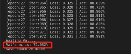
The accuracy of the training set is 88 and the verification set is only 72.6. There is no doubt that the model has some over fitting. The reason is that the amount of data is too small. A total of 2850 samples are divided into training set and verification set according to the ratio of 5:1. If you use transfer learning, you can use the pre training model to initialize the model, and then train, the effect should be much better.

3.3 transfer learning

As the name suggests, transfer learning is to transfer the trained model parameters to a new model to help the new model training. Considering that most data or tasks are relevant, we can share the learned model parameters (also known as the knowledge learned by the model) to the new model in some way through migration learning, so as to speed up and optimize the learning efficiency of the model, without learning from zero like most networks.

Advantages: 1 Speed up the training speed and lose converges quickly; 2. Over fitting can be reduced to obtain a model with stronger generalization ability.

Because the model defined by ourselves is different from resnet50 in the paper, it is impossible to directly load the online pre training model. Here, we use the restnet50 network provided by torchvision, then load the pre training model, change the last full connection layer, and then train. Just in train Py load the model here to modify it.

# 2. load model
    num_class = 14
    # model = ResNet50(Bottleneck,[3,4,6,3], num_class)
    model = models.resnet50(pretrained=True)
    fc_inputs = model.fc.in_features
    model.fc = nn.Linear(fc_inputs, num_class)
    device = torch.device('cuda' if torch.cuda.is_available() else 'cpu')
    model = model.to(device)

The final training results are as follows. When the epoch reaches 22, the loss is very small. The accuracy of the verification set is 88 and the accuracy of the training set is 99

Why is there such a big gap between zero learning and fine tune learning? The size of the loss function is ten times worse and the accuracy of the verification set is 20 times worse. Personally, I think it is more related to initialization. Initialization makes loss not rotate at a local minimum and finds a lower point, so the performance of the model is improved, but the problem of over fitting still exists.