Interested children, especially children's shoes, especially in the application of big data and artificial intelligence in quantification, can pay attention to my official account. If the script code is not clear, please see the official account number:
datahomex:

Through the introduction of the previous two articles in this series, we must have a basic understanding of procedural trading, but it is only procedural trading, not quantitative trading.
Today, datajun introduces you an open-source quantitative framework based on python, backtrader, which opens our formal learning path of quantitative trading.
1, Know backtrader
1.1 INTRODUCTION
backtrader official website:
Take a look at the introduction of backtrader on the official website:
A feature-rich Python framework for backtesting and trading
backtrader allows you to focus on writing reusable trading strategies, indicators and analyzers instead of having to spend time building infrastructure.
backtrader is an open source framework based on python for backtesting and trading. It enables users to focus on the development of trading strategies and indicators without caring about the infrastructure of the system.
In short, backtrader helps us set up the overall framework of quantitative trading and reserves rich interfaces for developers to use. It can support all links of quantitative trading, including data loading, policy development, policy backtracking and real-time trading.
1.2 components
backtrader core components:
1. Back test system (Cerebro):
-
It is necessary to set systematic parameters, such as initial capital, commission, trading position size, etc;
-
It is necessary to inject custom developed transaction strategies and test data sets;
2. Strategy:
The core part of quantitative trading development needs to develop buy and sell signals and design trading strategies;
3. Data Feed: the component of the test data set loaded into the back test system;
The above three are the core modules of backtrader in quantitative development. There are also some auxiliary components, such as plotting, built-in Indicators, Analyzers, LiveTrading, etc.
The functions and instructions of these components are described in detail on the official website. Of course, we will also introduce them one by one in the following series of articles.
2, Hello Algotrading!
We first use an introductory example given on the official website to appreciate the charm of the backtrade framework, execute the following script, and finally generate the performance of the trading strategy on the test data set.
2.1 interpretation of procedures
from datetime import datetime
import backtrader as bt

# Create a subclass of Strategy to define the indicators and logic

# The first step is to develop a custom Strategy, which needs to inherit the Strategy class of backtrader
class SmaCross(bt.Strategy):
    # list of parameters which are configurable for the strategy
    params = dict(
        pfast=10,  # period for the fast moving average
        pslow=30   # period for the slow moving average
    )
    # General log printing function, which can print orders and transaction records. It is optional and optional
    def log(self, txt, dt=None):
        dt = dt or self.datas[0].datetime.date(0)
        print('%s, %s' % (dt.isoformat(), txt))

	# The initialization function initializes the calculation of attributes and indicators. It is only executed once during the operation of the whole back test system
    def __init__(self):
        sma1 = bt.ind.SMA(period=self.p.pfast)  # fast moving average
        sma2 = bt.ind.SMA(period=self.p.pslow)  # slow moving average
        self.crossover = bt.ind.CrossOver(sma1, sma2)  # crossover signal

	# Order status message notification function
	def notify_order(self, order):
        if order.status in [order.Submitted, order.Accepted]:
            return
        # Check whether the order is completed
        if order.status in [order.Completed]:
            if order.isbuy():
                self.log(
                    'BUY EXECUTED, Price: %.2f, Cost: %.2f, Comm %.2f' %
                    (order.executed.price,
                     order.executed.value,
                     order.executed.comm))
            else:
                self.log('SELL EXECUTED, Price: %.2f, Cost: %.2f, Comm %.2f' %
                         (order.executed.price,
                          order.executed.value,
                          order.executed.comm))

	# Each trading day will be called in turn
    def next(self):
        if not self.position:  # not in the market
            if self.crossover > 0:  # if fast crosses slow to the upside
                self.buy()  # enter long

        elif self.crossover < 0:  # in the market & cross to the downside
            self.close()  # close long position

# Create a data feed
modpath = os.path.dirname(os.path.abspath(sys.argv[0]))
datapath = os.path.join(modpath,'603186.csv')
data = bt.feeds.GenericCSVData(
        dataname=datapath,
        fromdate=datetime.datetime(2010, 1, 1),
        todate=datetime.datetime(2020, 4, 12),
        dtformat='%Y%m%d',
        datetime=2,
        open=3,
        high=4,
        low=5,
        close=6,
        volume=10,
        reverse=True
    )

# The back test system is instantiated and translated into brain by Cerebro. The back test system is the control center of the whole backtrader
cerebro = bt.Cerebro()  # create a "Cerebro" engine instance
# Initial capital 10000
cerebro.broker.setcash(10000)
# commission
cerebro.broker.setcommission(commission=0.002)
cerebro.adddata(data)  # Add the data feed
cerebro.addstrategy(SmaCross)  # Add the trading strategy
cerebro.run()  # run it all
cerebro.plot()  # and plot it with a single command
Steps for using the backtrader framework:
1. The first step is to develop your own trading strategy class
class SmaCross(bt.Strategy)
The custom transaction strategy class needs to inherit bt.Strategy class. bt.Strategy class provides many methods for us to rewrite. Here are some of the most important functions:
init() function: initialization function. The back test process is only executed once. It is recommended to implement the one-time static indicators required by the strategy in this function, such as the long-term and short-term moving average indicators in the above example;
next() function: the core function, which will be called once every trading day. It is necessary to realize the trading order logic according to the trading signal of the day. For example, when the short-term moving average line crosses the long-term moving average line, buy and go long; Otherwise, sell and close the position.
Description of transaction function in Code:
self.buy(): buy long
self.sell(): sell short
In addition, common transaction functions:
self.close(): warehouse clearing
self.cancel(): cancel the order
notify_order function: order message notification function, which prints the order information of each transaction, including transaction price, transaction amount, commission, etc.
2. The second step is to prepare the back test data set
modpath = os.path.dirname(os.path.abspath(sys.argv[0]))
datapath = os.path.join(modpath,'orcl.txt')
data = bt.feeds.YahooFinanceCSVData(dataname= datapath,
                                 fromdate=datetime(2000, 1, 1),
                                 todate=datetime(2000, 12, 31))
With the strategy, we need the back test data set to test the effectiveness of our strategy. The backtrader framework has strict format requirements for the back test data set,
The default needs to include:
datetime, open, high, low, close, volume
The datafeeds data module in the backtrader supports many types of data forms, including third-party api, real-time data (Yahoo, VisualChart, Sierra Chart, Interactive Brokers, Yingtou, OANDA, Quandl), local txt, CSV files, pandas dataframe, incluxdb, MT4CSV, etc. the most commonly used third-party api may be the local file or dataframe.
If you have studied dbms (relational database), you can understand datafeeds as two-dimensional tables. If there is no database foundation, you can imagine it as excel tables. Each row represents the trading information of the stock on a trading day, and each column can be regarded as a line in the backtrader.
Many concepts of datafeeds in backtrader are still difficult to understand. We will explain them in detail later.
3. Create a back test system instance (straight white point can also be said to create a brain)
cerebro = bt.Cerebro() # create a "Cerebro" engine instance
After the back test instance is created, the transaction strategy and back test data are injected into the back test instance. You can also set the initial capital, commission and other information. Finally, the execution of the back test instance will print the transaction details of the whole transaction strategy on the test data set.
# Initial capital 10000
cerebro.broker.setcash(10000)
# commission
cerebro.broker.setcommission(commission=0.002)
# Back test data set
cerebro.adddata(data)  # Add the data feed
# Trading policy rate
cerebro.addstrategy(SmaCross)  # Add the trading strategy
2019-06-12, BUY EXECUTED, Price: 29.61, Cost: 2961.00, Comm 0.00
2019-10-10, SELL EXECUTED, Price: 39.79, Cost: 2961.00, Comm 0.00
2019-10-28, BUY EXECUTED, Price: 46.99, Cost: 4699.00, Comm 0.00
2019-11-20, SELL EXECUTED, Price: 43.00, Cost: 4699.00, Comm 0.00
2019-12-20, BUY EXECUTED, Price: 40.86, Cost: 4086.00, Comm 0.00
2019-12-24, SELL EXECUTED, Price: 38.64, Cost: 4086.00, Comm 0.00
2020-01-10, BUY EXECUTED, Price: 43.69, Cost: 4369.00, Comm 0.00
2020-03-23, SELL EXECUTED, Price: 49.00, Cost: 4369.00, Comm 0.00
2.2 interpretation of results
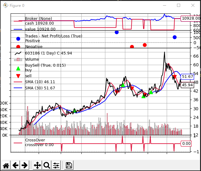
This simple trading strategy performed well, and the overall profit was unexpected. However, this is not the focus of our concern. Our focus is to introduce how to look at this figure:
1. The top part is the current cash and assets of the account. The red line represents the cash value and the blue line represents the total assets. You can see that the total cash of the total association is 10928
2. Below the K line, the red line is sma10, the blue line is sma30, and the red line is the closing price of the day
3. The red inverted triangle indicates selling short and the green triangle indicates buying long
4. The bottom part is the buying and selling signal line. When the value is greater than 0, it means that the short-term moving average uploads the long-term moving average to buy; When it is less than 0, it is sold.
3, Develop a custom policy
3.1 implement the entry strategy of the previous period
In the last issue, dataking developed a simple entry strategy. Let's use the backtrader framework to test it.
Buying signal: sma10 is worn on sma5. At that time, we obtained K-line data at the level of 5 minutes;
The selling signal satisfies any of the following conditions:
1) sma5 and sma10;
2) Current closing price > 1.01 * buying price and current (sma5-sma10) < previous period (sma5-sma10) * 0.95;
3) Current closing price < 0.97 * buying price;
# Implement the previous entry strategy
class SmaCross(bt.Strategy):
# list of parameters which are configurable for the strategy
params = dict(
pfast=10, # period for the fast moving average
pslow=30 # period for the slow moving average
)
# General log printing function, which can print orders and transaction records. It is optional and optional
def log(self, txt, dt=None):
dt = dt or self.datas[0].datetime.date(0)
print('%s, %s' % (dt.isoformat(), txt))
def notify_order(self, order):
if order.status in [order.Submitted, order.Accepted]:
return
if order.status in [order.Completed]:
if order.isbuy():
self.log('BUY EXECUTED, Price: %.2f, Cost: %.2f, Comm %.2f' %
(order.executed.price,
order.executed.value,
order.executed.comm))
self.buyprice = order.executed.price # Record cost price
else:
self.log('SELL EXECUTED, Price: %.2f, Cost: %.2f, Comm %.2f' %
(order.executed.price,
order.executed.value,
order.executed.comm))
return super().notify_order(order)
def __init__(self):
self.dataclose = self.datas[0].close
self.sma1 = bt.ind.SMA(period=self.p.pfast) # fast moving average
self.sma2 = bt.ind.SMA(period=self.p.pslow) # slow moving average
self.dif = self.sma1 - self.sma2
self.crossover = bt.ind.CrossOver(self.sma1, self.sma2) # crossover signal
self.buyprice = None # Purchase cost price
def next(self):
if not self.position: # not in the market
if self.crossover > 0: # if fast crosses slow to the upside
self.buy() # enter long
else:
condition = (self.dataclose[0] - self.buyprice) / self.dataclose[0]
if self.crossover < 0 or condition < 0.97 or (condition>1.01 and self.dif[0] < self.dif[-1] * 0.95) :
# in the market & cross to the downside
self.close(volume=False) # close long position
3.2 loading custom datasets
In [Article 1 coming children's shoes], the data master obtained the K-line data of 5 minutes level by calling the / market/history/kline interface and made local persistent storage. This time, we will use this part of data to test the above simple strategy back and forth. The specific code is as follows:
# Load data into model
from sqlalchemy import create_engine
import pandas as pd
import time
engine = create_engine('mysql://root:123456@127.0.0.1/stock?charset=utf8mb4')
conn = engine.connect()
sql=("select * from huobi_daily")
df = pd.read_sql(sql,engine)
df['date'] = df['id'].apply(lambda x:time.strftime('%Y-%m-%d %H:%M:%S', time.localtime(x)))
df['date'] = pd.to_datetime(df['date'])
df.index = df.date
data = bt.feeds.PandasData(dataname=df)
cerebro.adddata(data)
3.3 operation results
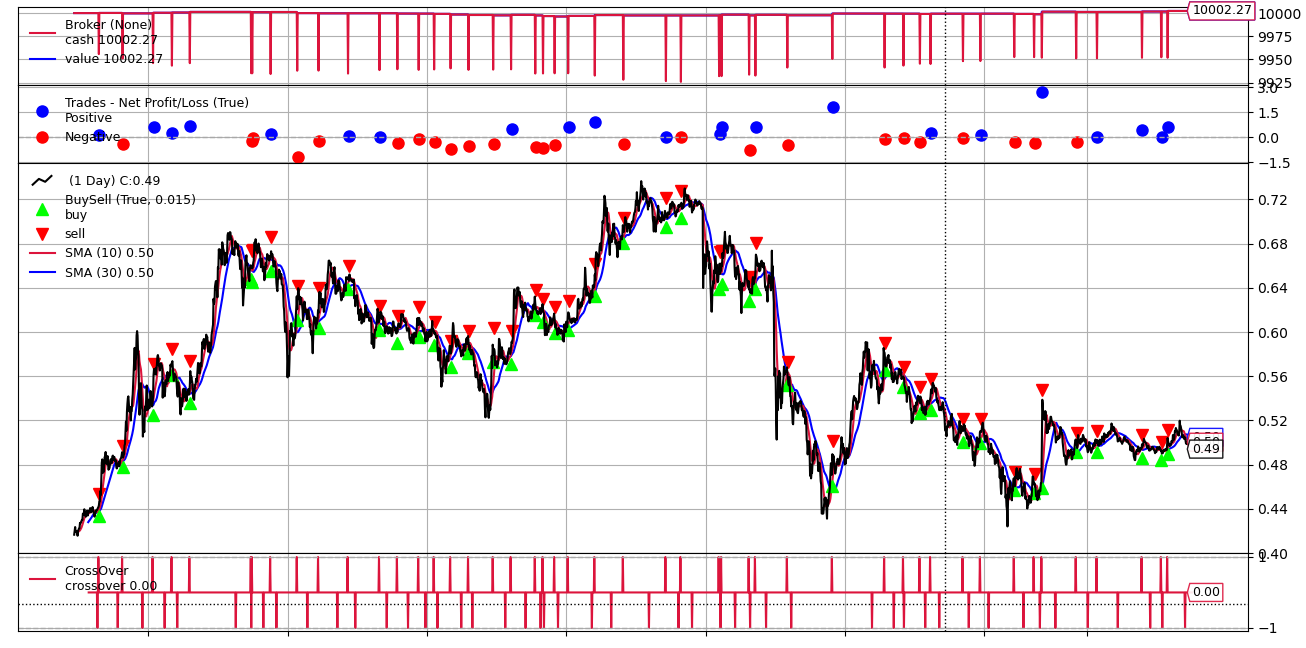
Summary:
Today, we have completed the development of a complete quantitative trading program. From the back test, the effect of our strategy in the previous period is very general in the short-term trading of several currencies. Of course, this is reasonable. After all, the strategy is too simple. Later, we will focus on the development of custom strategies, which may be combined with complex technologies such as statistical model, machine learning and deep learning, However, the whole framework and process are the same.
In addition, the backtrader framework introduced today will continue to be used later, and more functions and details will be explained at that time. I hope you can go further and further on the road of quantification with the data gentleman.