Introduction to ISLR statistical learning: R language code practice of linear regression

Posted by fleymingmasc on Fri, 28 Jan 2022 14:19:24 +0100

Chapter 2 linear regression

2.1 simple linear regression

The ISLR2 library contains the Boston dataset, which records medv (median house value) for 506 census districts in Boston.
We will use 12 predictive variables, such as rmvar (average number of rooms per household), age (average house age), and lstat (percentage of households with low socio-economic status), to predict medv.

library(ISLR2)
library(MASS)

head(Boston)

A data.frame: 6 × 14

	crim	zn	indus	chas	nox	rm	age	dis	rad	tax	ptratio	black	lstat	medv
	<dbl>	<dbl>	<dbl>	<int>	<dbl>	<dbl>	<dbl>	<dbl>	<int>	<dbl>	<dbl>	<dbl>	<dbl>	<dbl>
1	0.00632	18	2.31	0	0.538	6.575	65.2	4.0900	1	296	15.3	396.90	4.98	24.0
2	0.02731	0	7.07	0	0.469	6.421	78.9	4.9671	2	242	17.8	396.90	9.14	21.6
3	0.02729	0	7.07	0	0.469	7.185	61.1	4.9671	2	242	17.8	392.83	4.03	34.7
4	0.03237	0	2.18	0	0.458	6.998	45.8	6.0622	3	222	18.7	394.63	2.94	33.4
5	0.06905	0	2.18	0	0.458	7.147	54.2	6.0622	3	222	18.7	396.90	5.33	36.2
6	0.02985	0	2.18	0	0.458	6.430	58.7	6.0622	3	222	18.7	394.12	5.21	28.7

To learn more about datasets, we can type? Boston.
We will first use lm () function to fit a simple linear regression model,
medv was used as the explained variable and lstat was used as the explanatory variable.

lm.fit <- lm(medv~lstat, data = Boston)

lm.fit

Call:
lm(formula = medv ~ lstat, data = Boston)

Coefficients:
(Intercept)        lstat  
      34.55        -0.95

summary(lm.fit)

Call:
lm(formula = medv ~ lstat, data = Boston)

Residuals:
    Min      1Q  Median      3Q     Max 
-15.168  -3.990  -1.318   2.034  24.500 

Coefficients:
            Estimate Std. Error t value Pr(>|t|)    
(Intercept) 34.55384    0.56263   61.41   <2e-16 ***
lstat       -0.95005    0.03873  -24.53   <2e-16 ***
---
Signif. codes:  0 '***' 0.001 '**' 0.01 '*' 0.05 '.' 0.1 ' ' 1

Residual standard error: 6.216 on 504 degrees of freedom
Multiple R-squared:  0.5441,	Adjusted R-squared:  0.5432 
F-statistic: 601.6 on 1 and 504 DF,  p-value: < 2.2e-16

We can use the names () function to find out what other information is stored in lm. We can extract these quantities by name,
For example, LM Fit $coefficients, which are more secure to access using extractor functions such as coef ().

names(lm.fit)

'coefficients'
'residuals'
'effects'
'rank'
'fitted.values'
'assign'
'qr'
'df.residual'
'xlevels'
'call'
'terms'
'model'

# correlation coefficient
coef(lm.fit)

(Intercept) 34.5538408793831 lstat -0.95004935375799

# confidence interval
confint(lm.fit)

A matrix: 2 × 2 of type dbl

	2.5 %	97.5 %
(Intercept)	33.448457	35.6592247
lstat	-1.026148	-0.8739505

The predict() function can be used to generate confidence intervals and prediction intervals to predict the medv of a given lstat value.

predict(lm.fit, data.frame(lstat = c(5,10,15)), interval = 'prediction')

A matrix: 3 × 3 of type dbl

	fit	lwr	upr
1	29.80359	17.565675	42.04151
2	25.05335	12.827626	37.27907
3	20.30310	8.077742	32.52846

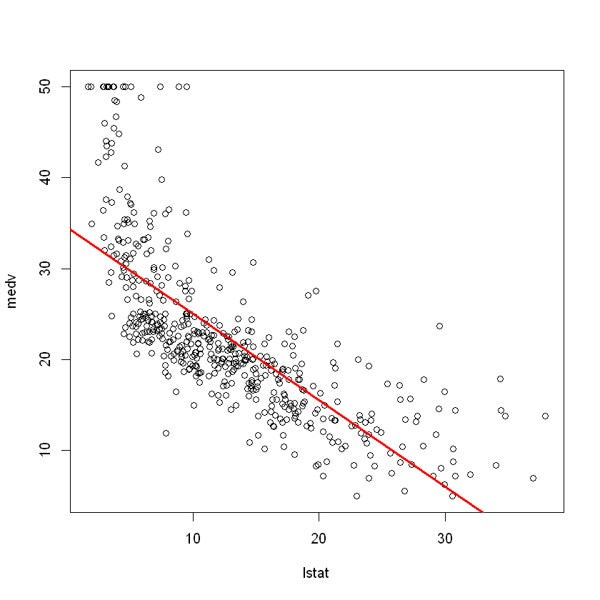
attach(Boston)
plot(lstat, medv)
abline(lm.fit)

The function is used to draw any straight line, not just the least squares regression line. To draw a line with intercept a and slope B, we need to type a line (a, b). Next, we'll experiment with some additional settings for lines and points. The lwd=3 command increases the width of the regression line by 3 times;
This also applies to the plot () and lines () functions. We can also use the pch option to create different symbols.

plot(lstat, medv)
abline(lm.fit, lwd = 3, col='red')

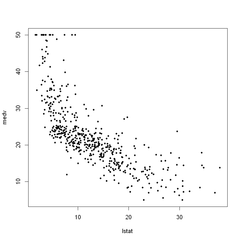
plot(lstat, medv, pch = 20)

plot(lstat, medv, pch = "+")

plot(1:20, 1:20, pch = 1:20)

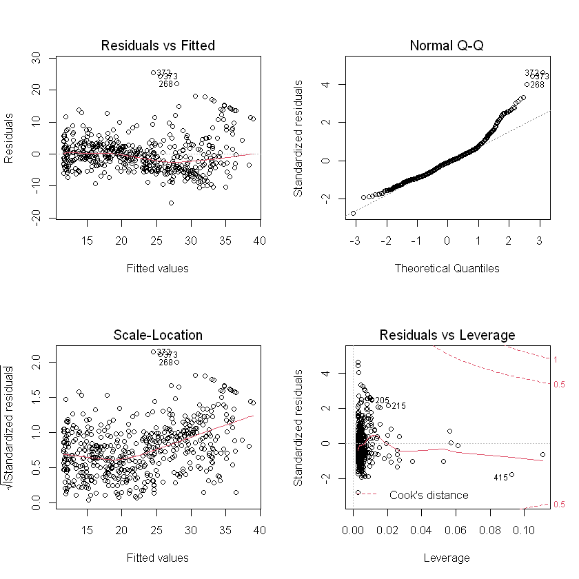
par(mfrow = c(2, 2))
plot(lm.fit)

which.max(hatvalues(lm.fit))

375: 375

which. The max() function identifies the index of the largest element in the vector. In this case, it tells us which observation has the largest leverage statistics.

2.2 multiple linear regression

In order to use the least square method to fit the multiple linear regression model, we use the lm () function again, and the summary () function now outputs the regression coefficients of all predicted values.

mfit <- lm(medv~lstat + age)
summary(mfit)

Call:
lm(formula = medv ~ lstat + age)

Residuals:
    Min      1Q  Median      3Q     Max 
-15.981  -3.978  -1.283   1.968  23.158 

Coefficients:
            Estimate Std. Error t value Pr(>|t|)    
(Intercept) 33.22276    0.73085  45.458  < 2e-16 ***
lstat       -1.03207    0.04819 -21.416  < 2e-16 ***
age          0.03454    0.01223   2.826  0.00491 ** 
---
Signif. codes:  0 '***' 0.001 '**' 0.01 '*' 0.05 '.' 0.1 ' ' 1

Residual standard error: 6.173 on 503 degrees of freedom
Multiple R-squared:  0.5513,	Adjusted R-squared:  0.5495 
F-statistic:   309 on 2 and 503 DF,  p-value: < 2.2e-16

The Boston data set contains 12 variables, so it will be troublesome to type all these variables in order to use all the predicted values for regression. Instead, we can use the following abbreviations:

lm.fit <- lm(medv ~ ., data = Boston)
summary(lm.fit)

Call:
lm(formula = medv ~ ., data = Boston)

Residuals:
    Min      1Q  Median      3Q     Max 
-15.595  -2.730  -0.518   1.777  26.199 

Coefficients:
              Estimate Std. Error t value Pr(>|t|)    
(Intercept)  3.646e+01  5.103e+00   7.144 3.28e-12 ***
crim        -1.080e-01  3.286e-02  -3.287 0.001087 ** 
zn           4.642e-02  1.373e-02   3.382 0.000778 ***
indus        2.056e-02  6.150e-02   0.334 0.738288    
chas         2.687e+00  8.616e-01   3.118 0.001925 ** 
nox         -1.777e+01  3.820e+00  -4.651 4.25e-06 ***
rm           3.810e+00  4.179e-01   9.116  < 2e-16 ***
age          6.922e-04  1.321e-02   0.052 0.958229    
dis         -1.476e+00  1.995e-01  -7.398 6.01e-13 ***
rad          3.060e-01  6.635e-02   4.613 5.07e-06 ***
tax         -1.233e-02  3.760e-03  -3.280 0.001112 ** 
ptratio     -9.527e-01  1.308e-01  -7.283 1.31e-12 ***
black        9.312e-03  2.686e-03   3.467 0.000573 ***
lstat       -5.248e-01  5.072e-02 -10.347  < 2e-16 ***
---
Signif. codes:  0 '***' 0.001 '**' 0.01 '*' 0.05 '.' 0.1 ' ' 1

Residual standard error: 4.745 on 492 degrees of freedom
Multiple R-squared:  0.7406,	Adjusted R-squared:  0.7338 
F-statistic: 108.1 on 13 and 492 DF,  p-value: < 2.2e-16

summary(lm.fit)$r.sq$ R 2 {R^2} R2, (lm.fit) $sigma provides us with RSE. The Vif () function is part of the car package and can be used to calculate the variance expansion coefficient.

library(car)

Warning message:
"package 'car' was built under R version 4.0.5"
Loading required package: carData

Warning message:
"package 'carData' was built under R version 4.0.3"

vif(lm.fit)

crim 1.79219154743324 zn 2.29875817874944 indus 3.99159641834602 chas 1.07399532755379 nox 4.39371984757748 rm 1.93374443578326 age 3.10082551281533 dis 3.95594490637272 rad 7.48449633527445 tax 9.00855394759706 ptratio 1.79908404924889 black 1.34852107640637 lstat 2.94149107809193

What if we want to perform regression with all variables except one? For example, in the above regression output, age has a higher p value. Therefore, we may want to run a regression that does not include this prediction. The following syntax leads to regression using all predictors except age.

mfit2 <- lm(medv ~.- age, data=Boston)
summary(mfit2)

Call:
lm(formula = medv ~ . - age, data = Boston)

Residuals:
     Min       1Q   Median       3Q      Max 
-15.6054  -2.7313  -0.5188   1.7601  26.2243 

Coefficients:
              Estimate Std. Error t value Pr(>|t|)    
(Intercept)  36.436927   5.080119   7.172 2.72e-12 ***
crim         -0.108006   0.032832  -3.290 0.001075 ** 
zn            0.046334   0.013613   3.404 0.000719 ***
indus         0.020562   0.061433   0.335 0.737989    
chas          2.689026   0.859598   3.128 0.001863 ** 
nox         -17.713540   3.679308  -4.814 1.97e-06 ***
rm            3.814394   0.408480   9.338  < 2e-16 ***
dis          -1.478612   0.190611  -7.757 5.03e-14 ***
rad           0.305786   0.066089   4.627 4.75e-06 ***
tax          -0.012329   0.003755  -3.283 0.001099 ** 
ptratio      -0.952211   0.130294  -7.308 1.10e-12 ***
black         0.009321   0.002678   3.481 0.000544 ***
lstat        -0.523852   0.047625 -10.999  < 2e-16 ***
---
Signif. codes:  0 '***' 0.001 '**' 0.01 '*' 0.05 '.' 0.1 ' ' 1

Residual standard error: 4.74 on 493 degrees of freedom
Multiple R-squared:  0.7406,	Adjusted R-squared:  0.7343 
F-statistic: 117.3 on 12 and 493 DF,  p-value: < 2.2e-16

2.3 interactive items

The lm () function makes it easy to include interaction terms in a linear model. Syntax lstat:black tells R to include an interaction item between lstat and black. The syntax lstat*age includes lstat, age and interactive item lstat at the same time × Age as predictor; It is the abbreviation of lstat+age+lstat:age. We can also pass the converted prediction value.

summary(lm(medv ~ lstat * age, data = Boston))

Call:
lm(formula = medv ~ lstat * age, data = Boston)

Residuals:
    Min      1Q  Median      3Q     Max 
-15.806  -4.045  -1.333   2.085  27.552 

Coefficients:
              Estimate Std. Error t value Pr(>|t|)    
(Intercept) 36.0885359  1.4698355  24.553  < 2e-16 ***
lstat       -1.3921168  0.1674555  -8.313 8.78e-16 ***
age         -0.0007209  0.0198792  -0.036   0.9711    
lstat:age    0.0041560  0.0018518   2.244   0.0252 *  
---
Signif. codes:  0 '***' 0.001 '**' 0.01 '*' 0.05 '.' 0.1 ' ' 1

Residual standard error: 6.149 on 502 degrees of freedom
Multiple R-squared:  0.5557,	Adjusted R-squared:  0.5531 
F-statistic: 209.3 on 3 and 502 DF,  p-value: < 2.2e-16

2.4 nonlinear conversion

lm () function can also be used for nonlinear transformation of explanatory variables.
For example, given an explanatory variable X, we can use I (X2) to create ${X^2} $. The function I () is required because it has special meaning in the formula object;
Our packaging allows the use of standard usage in R, that is, raising X to a power of 2. We will now return medv to lstat and lstat^2.

lm.fit2 <- lm(medv ~ lstat + I(lstat^2))
summary(lm.fit2)

Call:
lm(formula = medv ~ lstat + I(lstat^2))

Residuals:
     Min       1Q   Median       3Q      Max 
-15.2834  -3.8313  -0.5295   2.3095  25.4148 

Coefficients:
             Estimate Std. Error t value Pr(>|t|)    
(Intercept) 42.862007   0.872084   49.15   <2e-16 ***
lstat       -2.332821   0.123803  -18.84   <2e-16 ***
I(lstat^2)   0.043547   0.003745   11.63   <2e-16 ***
---
Signif. codes:  0 '***' 0.001 '**' 0.01 '*' 0.05 '.' 0.1 ' ' 1

Residual standard error: 5.524 on 503 degrees of freedom
Multiple R-squared:  0.6407,	Adjusted R-squared:  0.6393 
F-statistic: 448.5 on 2 and 503 DF,  p-value: < 2.2e-16

# The two models are compared by analysis of variance
lm.fit <- lm(medv ~ lstat)
anova(lm.fit, lm.fit2)

A anova: 2 × 6

	Res.Df	RSS	Df	Sum of Sq	F	Pr(>F)
	<dbl>	<dbl>	<dbl>	<dbl>	<dbl>	<dbl>
1	504	19472.38	NA	NA	NA	NA
2	503	15347.24	1	4125.138	135.1998	7.630116e-28

Here, model 1 represents a linear sub model containing only one explanatory variable lstat, while model 2 corresponds to a quadratic model with two explanatory variables lstat and lstat^2. The function is used to test the hypothesis of the two models.
The null hypothesis is that both models can fit the data well, and the selected hypothesis is that the whole model is better. Here, the statistical value of F is 135 and the value of p is almost zero. This provides very clear evidence that the model containing lstat and lstat^2 is much better than the model containing only lstat. This is not surprising because earlier we saw nonlinear evidence of the relationship between medv and lstat

par(mfrow = c(2, 2))
plot(lm.fit2)

And then we see, when l s t a t 2 lstat^2 When lstat2 item is included in the model, it performs better in the residual diagram. To create a cubic fit, we can include predictions of form I (X^3). However, for higher-order polynomials, this method may begin to become troublesome. A better approach is to use the poly () function to create polynomials in lm (). For example, the following command generates a fifth order polynomial fit:

mfit5 <- lm(medv ~ poly(lstat, 5))
summary(mfit5)

Call:
lm(formula = medv ~ poly(lstat, 5))

Residuals:
     Min       1Q   Median       3Q      Max 
-13.5433  -3.1039  -0.7052   2.0844  27.1153 

Coefficients:
                 Estimate Std. Error t value Pr(>|t|)    
(Intercept)       22.5328     0.2318  97.197  < 2e-16 ***
poly(lstat, 5)1 -152.4595     5.2148 -29.236  < 2e-16 ***
poly(lstat, 5)2   64.2272     5.2148  12.316  < 2e-16 ***
poly(lstat, 5)3  -27.0511     5.2148  -5.187 3.10e-07 ***
poly(lstat, 5)4   25.4517     5.2148   4.881 1.42e-06 ***
poly(lstat, 5)5  -19.2524     5.2148  -3.692 0.000247 ***
---
Signif. codes:  0 '***' 0.001 '**' 0.01 '*' 0.05 '.' 0.1 ' ' 1

Residual standard error: 5.215 on 500 degrees of freedom
Multiple R-squared:  0.6817,	Adjusted R-squared:  0.6785 
F-statistic: 214.2 on 5 and 500 DF,  p-value: < 2.2e-16

This shows that including additional polynomial terms up to fifth order can improve model fitting! However, the further study of the data shows that the polynomial terms above the fifth order have no significant p value in the regression fitting.

# Logarithmic transformation
summary(lm(medv ~ log(rm), data = Boston))

Call:
lm(formula = medv ~ log(rm), data = Boston)

Residuals:
    Min      1Q  Median      3Q     Max 
-19.487  -2.875  -0.104   2.837  39.816 

Coefficients:
            Estimate Std. Error t value Pr(>|t|)    
(Intercept)  -76.488      5.028  -15.21   <2e-16 ***
log(rm)       54.055      2.739   19.73   <2e-16 ***
---
Signif. codes:  0 '***' 0.001 '**' 0.01 '*' 0.05 '.' 0.1 ' ' 1

Residual standard error: 6.915 on 504 degrees of freedom
Multiple R-squared:  0.4358,	Adjusted R-squared:  0.4347 
F-statistic: 389.3 on 1 and 504 DF,  p-value: < 2.2e-16

2.5 qualitative explanatory variables

Now we will examine the Carseats data, which is part of the ISLR2 library. We will try to predict sales in 400 locations based on some explanatory variables.

head(Carseats)

A data.frame: 6 × 11

	Sales	CompPrice	Income	Advertising	Population	Price	ShelveLoc	Age	Education	Urban	US
	<dbl>	<dbl>	<dbl>	<dbl>	<dbl>	<dbl>	<fct>	<dbl>	<dbl>	<fct>	<fct>
1	9.50	138	73	11	276	120	Bad	42	17	Yes	Yes
2	11.22	111	48	16	260	83	Good	65	10	Yes	Yes
3	10.06	113	35	10	269	80	Medium	59	12	Yes	Yes
4	7.40	117	100	4	466	97	Medium	55	14	Yes	Yes
5	4.15	141	64	3	340	128	Bad	38	13	Yes	No
6	10.81	124	113	13	501	72	Bad	78	16	No	Yes

Car seat data includes qualitative predictors, such as shelveloc, which is an indicator of shelf position quality, that is, each position in the store shows the space of car seats. The predictor shelleloc has three possible values: bad, medium, and good. Given a qualitative variable (such as shelveloc), R will automatically generate a virtual variable. Next, we fit a multiple regression model, including some interaction terms.

lm.fit <- lm(Sales ~ . + Income:Advertising + Price:Age, 
    data = Carseats)
summary(lm.fit)

Call:
lm(formula = Sales ~ . + Income:Advertising + Price:Age, data = Carseats)

Residuals:
    Min      1Q  Median      3Q     Max 
-2.9208 -0.7503  0.0177  0.6754  3.3413 

Coefficients:
                     Estimate Std. Error t value Pr(>|t|)    
(Intercept)         6.5755654  1.0087470   6.519 2.22e-10 ***
CompPrice           0.0929371  0.0041183  22.567  < 2e-16 ***
Income              0.0108940  0.0026044   4.183 3.57e-05 ***
Advertising         0.0702462  0.0226091   3.107 0.002030 ** 
Population          0.0001592  0.0003679   0.433 0.665330    
Price              -0.1008064  0.0074399 -13.549  < 2e-16 ***
ShelveLocGood       4.8486762  0.1528378  31.724  < 2e-16 ***
ShelveLocMedium     1.9532620  0.1257682  15.531  < 2e-16 ***
Age                -0.0579466  0.0159506  -3.633 0.000318 ***
Education          -0.0208525  0.0196131  -1.063 0.288361    
UrbanYes            0.1401597  0.1124019   1.247 0.213171    
USYes              -0.1575571  0.1489234  -1.058 0.290729    
Income:Advertising  0.0007510  0.0002784   2.698 0.007290 ** 
Price:Age           0.0001068  0.0001333   0.801 0.423812    
---
Signif. codes:  0 '***' 0.001 '**' 0.01 '*' 0.05 '.' 0.1 ' ' 1

Residual standard error: 1.011 on 386 degrees of freedom
Multiple R-squared:  0.8761,	Adjusted R-squared:  0.8719 
F-statistic:   210 on 13 and 386 DF,  p-value: < 2.2e-16

The contrasts() function returns a dummy variable

attach(Carseats)
contrasts(ShelveLoc)

A matrix: 3 × 2 of type dbl

	Good	Medium
Bad	0	0
Good	1	0
Medium	0	1

R creates a ShelveLocGood dummy variable. If the shelving position is good, the value of the variable is 1, otherwise it is 0. It also creates a ShelveLocMedium dummy variable. If the shelving position is medium, the variable is equal to 1, otherwise it is 0. The wrong shelving position corresponds to the zero of each of the two dummy variables. The fact that the shelf commodity coefficient in the regression output is positive shows that good shelf position is related to higher sales (relative to bad position). The positive coefficient of ShelveLocMedium is small, indicating that the sales of medium shelf position is higher than that of poor shelf position, but lower than that of good shelf position.

2.6 function writing

As we can see, R comes with many useful functions, and more functions can be obtained through the R library. However, we are usually interested in performing an operation that does not have a function that can be used directly. In this setup, we may need to write our own functions. For example, below we provide a simple function called LoadLibraries (), which is used to read ISLR2 and MASS libraries. Before we create the function, if we try to call it, R will return an error.

LoadLibraries <- function(){
    library(ISLR2)
    library(MASS)
    print("Related libraries have been imported")
}

LoadLibraries()

[1] "Related libraries have been imported"

Topics: R Language Algorithm

Programmer Think