I Linear regression
1. lm() function returns the prediction model of input variables, and the returned results can be used with many functions.
> lm.model <- lm(wt ~ mpg, data = mtcars)


> coefficients(lm.model) # Extraction coefficient
(Intercept)         mpg
   6.047255   -0.140862

> confint(lm.model, level=0.95) # After the distribution of the correlation coefficient of the linear model is obtained, the interval is limited to obtain the value of the boundary point
                 2.5 %     97.5 %
(Intercept)  5.4168245  6.6776856
mpg         -0.1709569 -0.1107671


> fitted(lm.model) # Use the established model to predict wt
          Mazda RX4       Mazda RX4 Wag          Datsun 710      Hornet 4 Drive   Hornet Sportabout             Valiant          Duster 360
           3.089154            3.089154            2.835602            3.032809            3.413136            3.497653            4.032929
          Merc 240D            Merc 230            Merc 280           Merc 280C          Merc 450SE          Merc 450SL         Merc 450SLC
           2.610223            2.835602            3.342705            3.539912            3.737119            3.610343            3.906153
 Cadillac Fleetwood Lincoln Continental   Chrysler Imperial            Fiat 128         Honda Civic      Toyota Corolla       Toyota Corona
           4.582291            4.582291            3.976584            1.483327            1.765051            1.272034            3.018723
   Dodge Challenger         AMC Javelin          Camaro Z28    Pontiac Firebird           Fiat X1-9       Porsche 914-2        Lotus Europa
           3.863894            3.906153            4.173791            3.342705            2.201723            2.384844            1.765051
     Ford Pantera L        Ferrari Dino       Maserati Bora          Volvo 142E
           3.821636            3.272274            3.934325            3.032809


> residuals(lm.model) # Residual between prediction and reality
          Mazda RX4       Mazda RX4 Wag          Datsun 710      Hornet 4 Drive   Hornet Sportabout             Valiant          Duster 360
        -0.46915365         -0.21415365         -0.51560210          0.18219114          0.02686382         -0.03765336         -0.46292884
          Merc 240D            Merc 230            Merc 280           Merc 280C          Merc 450SE          Merc 450SL         Merc 450SLC
         0.57977705          0.31439790          0.09729481         -0.09991195          0.33288129          0.11965707         -0.12615307
 Cadillac Fleetwood Lincoln Continental   Chrysler Imperial            Fiat 128         Honda Civic      Toyota Corolla       Toyota Corona
         0.66770947          0.84170947          1.36841594          0.71667281         -0.15005113          0.56296577         -0.55372266
   Dodge Challenger         AMC Javelin          Camaro Z28    Pontiac Firebird           Fiat X1-9       Porsche 914-2        Lotus Europa
        -0.34389448         -0.47115307         -0.33379081          0.50229481         -0.26672324         -0.24484380         -0.25205113
     Ford Pantera L        Ferrari Dino       Maserati Bora          Volvo 142E
        -0.65163589         -0.50227421         -0.36432547         -0.25280886


> anova(lm.model) # anova table
Analysis of Variance Table

Response: wt
          Df  Sum Sq Mean Sq F value    Pr(>F)
mpg        1 22.3431 22.3431  91.375 1.294e-10 ***
Residuals 30  7.3356  0.2445
---
Signif. codes:  0 '***' 0.001 '**' 0.01 '*' 0.05 '.' 0.1 ' ' 1


> vcov(lm.model) # covariance matrix
             (Intercept)           mpg
(Intercept)  0.095289963 -0.0043626666
mpg         -0.004362667  0.0002171494


> influence(lm.model) # It is equivalent to a summary of the results of the analysis
$hat
          Mazda RX4       Mazda RX4 Wag          Datsun 710      Hornet 4 Drive   Hornet Sportabout             Valiant          Duster 360
         0.03198439          0.03198439          0.03776901          0.03277255          0.03296737          0.03476902          0.06102792
          Merc 240D            Merc 230            Merc 280           Merc 280C          Merc 450SE          Merc 450SL         Merc 450SLC
         0.04774195          0.03776901          0.03195442          0.03590963          0.04334604          0.03816586          0.05249086
 Cadillac Fleetwood Lincoln Continental   Chrysler Imperial            Fiat 128         Honda Civic      Toyota Corolla       Toyota Corona
         0.11464634          0.11464634          0.05705606          0.16580983          0.12563611          0.20060244          0.03301399
   Dodge Challenger         AMC Javelin          Camaro Z28    Pontiac Firebird           Fiat X1-9       Porsche 914-2        Lotus Europa
         0.04996488          0.05249086          0.07220085          0.03195442          0.07740711          0.06226177          0.12563611
     Ford Pantera L        Ferrari Dino       Maserati Bora          Volvo 142E
         0.04759875          0.03138551          0.05426366          0.03277255

$coefficients
                     (Intercept)           mpg
Mazda RX4           -0.007282030 -3.913985e-04
Mazda RX4 Wag       -0.003324014 -1.786609e-04
Datsun 710           0.009157470 -1.289282e-03
Hornet 4 Drive       0.001485910  2.190313e-04
Hornet Sportabout    0.001557359 -3.430679e-05
Valiant             -0.002604528  6.896128e-05
Duster 360          -0.066342655  2.535306e-03
Merc 240D           -0.027785644  2.330044e-03
Merc 230            -0.005583936  7.861634e-04
Merc 280             0.004737902 -7.949360e-05
Merc 280C           -0.007473905  2.108129e-04
Merc 450SE           0.033786317 -1.140454e-03
Merc 450SL           0.010081735 -3.083068e-04
Merc 450SLC         -0.015778260  5.782587e-04
Cadillac Fleetwood   0.153962430 -6.490318e-03
Lincoln Continental  0.194083866 -8.181645e-03
Chrysler Imperial    0.184925710 -6.947280e-03
Fiat 128            -0.161833613  9.391507e-03
Honda Civic          0.026202892 -1.571169e-03
Toyota Corolla      -0.151504789  8.636477e-03
Toyota Corona       -0.003495500 -7.167077e-04
Dodge Challenger    -0.040959820  1.475709e-03
AMC Javelin         -0.058928219  2.159665e-03
Camaro Z28          -0.054830702  2.169570e-03
Pontiac Firebird     0.024459924 -4.103942e-04
Fiat X1-9            0.028152063 -1.850938e-03
Porsche 914-2        0.019369325 -1.370227e-03
Lotus Europa         0.044014788 -2.639199e-03
Ford Pantera L      -0.073758568  2.607048e-03
Ferrari Dino        -0.019818649  1.798843e-04
Maserati Bora       -0.047027088  1.741542e-03
Volvo 142E          -0.002061852 -3.039283e-04

$sigma
          Mazda RX4       Mazda RX4 Wag          Datsun 710      Hornet 4 Drive   Hornet Sportabout             Valiant          Duster 360
          0.4950874           0.5013168           0.4933815           0.5017657           0.5029179           0.5028932           0.4950577
          Merc 240D            Merc 230            Merc 280           Merc 280C          Merc 450SE          Merc 450SL         Merc 450SLC
          0.4906934           0.4994096           0.5026082           0.5025884           0.4989569           0.5024330           0.5023674
 Cadillac Fleetwood Lincoln Continental   Chrysler Imperial            Fiat 128         Honda Civic      Toyota Corolla       Toyota Corona
          0.4853738           0.4747194           0.4295043           0.4813738           0.5020600           0.4891637           0.4919538
   Dodge Challenger         AMC Javelin          Camaro Z28    Pontiac Firebird           Fiat X1-9       Porsche 914-2        Lotus Europa
          0.4986579           0.4948469           0.4988098           0.4939281           0.5002931           0.5007472           0.5004465
     Ford Pantera L        Ferrari Dino       Maserati Bora          Volvo 142E
          0.4874197           0.4939342           0.4981090           0.5006732

$wt.res
          Mazda RX4       Mazda RX4 Wag          Datsun 710      Hornet 4 Drive   Hornet Sportabout             Valiant          Duster 360
        -0.46915365         -0.21415365         -0.51560210          0.18219114          0.02686382         -0.03765336         -0.46292884
          Merc 240D            Merc 230            Merc 280           Merc 280C          Merc 450SE          Merc 450SL         Merc 450SLC
         0.57977705          0.31439790          0.09729481         -0.09991195          0.33288129          0.11965707         -0.12615307
 Cadillac Fleetwood Lincoln Continental   Chrysler Imperial            Fiat 128         Honda Civic      Toyota Corolla       Toyota Corona
         0.66770947          0.84170947          1.36841594          0.71667281         -0.15005113          0.56296577         -0.55372266
   Dodge Challenger         AMC Javelin          Camaro Z28    Pontiac Firebird           Fiat X1-9       Porsche 914-2        Lotus Europa
        -0.34389448         -0.47115307         -0.33379081          0.50229481         -0.26672324         -0.24484380         -0.25205113
     Ford Pantera L        Ferrari Dino       Maserati Bora          Volvo 142E
        -0.65163589         -0.50227421         -0.36432547         -0.25280886
2. Evaluation of fitting quality
(1) The predicted value is obtained according to the model
predict(model, For training generation model Data set of)
(2) Use the R2 function in the caret package
R2(predict As a result, in the original dataset y value)
II multiple linear regression
1. Analysis of LM () and interaction
(1) Directly enter multiple variables into fomular and connect them with a plus sign:
mtcars.m <- lm(wt~mpg+disp+mpg:disp, data = mtcars)

##Analyze the model of independent variable disp and mpg to dependent variable wt, where mpg:disp means that the interaction between the two variables is considered when constructing the linear model
##That is, the two variables are not independent of each other

summary(mtcars.m)
Model:
> summary(mtcars.m)

Call:
lm(formula = wt ~ mpg + disp + mpg:disp, data = mtcars)

Residuals:
    Min      1Q  Median      3Q     Max
-0.8047 -0.2636  0.0539  0.2340  0.8817

Coefficients:
              Estimate Std. Error t value Pr(>|t|)
(Intercept)  3.3716803  0.7066020   4.772 5.18e-05 ***
mpg         -0.0505361  0.0257971  -1.959  0.06014 .
disp         0.0065258  0.0020525   3.179  0.00359 **
mpg:disp    -0.0001603  0.0001232  -1.301  0.20383
---
Signif. codes:  0 '***' 0.001 '**' 0.01 '*' 0.05 '.' 0.1 ' ' 1

Residual standard error: 0.4055 on 28 degrees of freedom
Multiple R-squared:  0.8449,	Adjusted R-squared:  0.8283
F-statistic: 50.84 on 3 and 28 DF,  p-value: 1.871e-11
(2) influence weight of independent variable
Count the "importance" of different variables to the model:
library(relaimpo);
calc.relimp( wt~mpg+disp+mpg:disp, data = mtcars )
> calc.relimp( wt~mpg+disp+mpg:disp, data = mtcars )
Response variable: wt
Total response variance: 0.957379
Analysis based on 32 observations
3 Regressors:
mpg disp mpg:disp
Proportion of variance explained by model: 84.49%
Metrics are not normalized (rela=FALSE).
Relative importance metrics: ##Influence weight
lmg
mpg 0.399914296
disp 0.435589844
mpg:disp 0.009378141
Average coefficients for different model sizes:
1X 2Xs 3Xs
mpg -0.140861970 -0.066315339 -0.0505361268
disp 0.007010325 0.004277131 0.0065257929
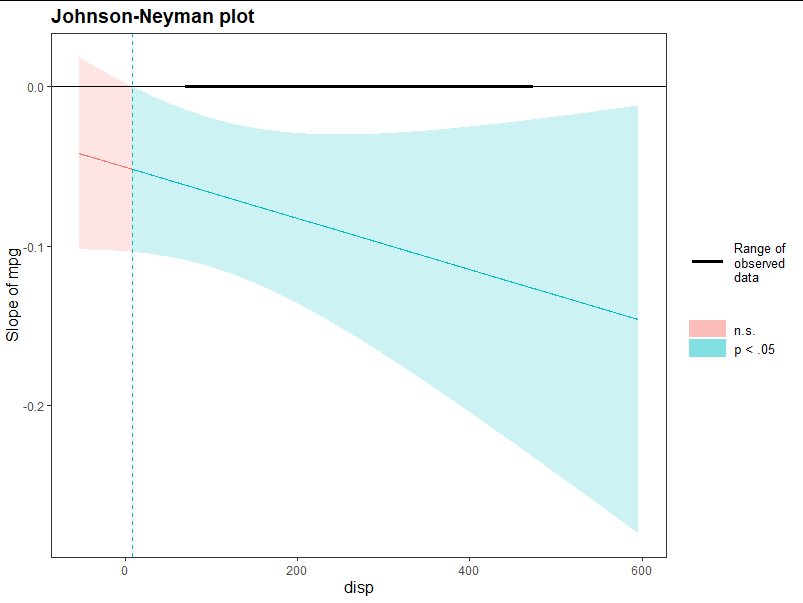
mpg:disp NaN NaN -0.0001603097(3) Visualize how independent variables affect each other
The interaction is mainly reflected in the change of slope:
library(interactions)
sim_slopes(mtcars.m, pred = mpg, modx = disp, jnplot = TRUE)
##pred input affected amount modx input affected amount
Results:
JOHNSON-NEYMAN INTERVAL

When disp is INSIDE the interval [8.39, 747.98], the slope of mpg is p < .05.

Note: The range of observed values of disp is [71.10, 472.00]

SIMPLE SLOPES ANALYSIS

##Random access to data, the results are somewhat outrageous
2. glm()
When the parameter famil y = "Gaussian" in glm function, your fitting effect is consistent with lm(), but glm can also be used in other regression models, such as linear regression in binary classification:
##glm is used to establish a linear model for the variables in swiss. When different independent variables are input, we can judge the corresponding specifications type through the numerical results

dat <- iris %>% filter( Species %in% c("setosa", "virginica") )
dat$Species <- as.factor(dat$Species)##The column corresponding to "dependent variable" needs to be processed, otherwise an error may be reported

bm <- glm( Species ~ Sepal.Length + Sepal.Width + Petal.Length + Petal.Width,
data = dat, family = binomial )  ##Select the model of binomial distribution

mtcars.predict1 <- predict(bm, dat,type = "response")
mtcars.predict2 <- predict(bm, dat) ##Use the default type
Results: note that the response model is set, and the output value has the effect of binary classification
> mtcars.predict1
           1            2            3            4            5            6            7            8            9           10           11           12
2.220446e-16 4.732528e-13 1.369834e-13 3.388726e-12 2.220446e-16 3.892826e-13 7.748530e-13 1.988060e-13 5.204109e-12 3.900993e-13 2.220446e-16 1.453927e-12
          13           14           15           16           17           18           19           20           21           22           23           24
2.656364e-13 2.220446e-16 2.220446e-16 2.220446e-16 2.220446e-16 2.220446e-16 2.220446e-16 2.220446e-16 4.472442e-13 2.682276e-13 2.220446e-16 4.132652e-11
          25           26           27           28           29           30           31           32           33           34           35           36
5.282004e-11 3.493413e-12 4.614812e-12 2.220446e-16 2.220446e-16 4.976501e-12 5.082694e-12 2.857677e-13 2.220446e-16 2.220446e-16 1.032749e-12 2.220446e-16
          37           38           39           40           41           42           43           44           45           46           47           48
2.220446e-16 2.220446e-16 1.035326e-12 1.337875e-13 2.220446e-16 3.421128e-11 4.494793e-13 2.131127e-11 2.126479e-11 1.861773e-12 2.220446e-16 6.741667e-13
          49           50           51           52           53           54           55           56           57           58           59           60
2.220446e-16 2.220446e-16 1.000000e+00 1.000000e+00 1.000000e+00 1.000000e+00 1.000000e+00 1.000000e+00 1.000000e+00 1.000000e+00 1.000000e+00 1.000000e+00
          61           62           63           64           65           66           67           68           69           70           71           72
1.000000e+00 1.000000e+00 1.000000e+00 1.000000e+00 1.000000e+00 1.000000e+00 1.000000e+00 1.000000e+00 1.000000e+00 1.000000e+00 1.000000e+00 1.000000e+00
          73           74           75           76           77           78           79           80           81           82           83           84
1.000000e+00 1.000000e+00 1.000000e+00 1.000000e+00 1.000000e+00 1.000000e+00 1.000000e+00 1.000000e+00 1.000000e+00 1.000000e+00 1.000000e+00 1.000000e+00
          85           86           87           88           89           90           91           92           93           94           95           96
1.000000e+00 1.000000e+00 1.000000e+00 1.000000e+00 1.000000e+00 1.000000e+00 1.000000e+00 1.000000e+00 1.000000e+00 1.000000e+00 1.000000e+00 1.000000e+00
          97           98           99          100
1.000000e+00 1.000000e+00 1.000000e+00 1.000000e+00
> mtcars.predict2
        1         2         3         4         5         6         7         8         9        10        11        12        13        14        15
-31.25726 -28.37915 -29.61892 -26.41057 -31.27837 -28.57447 -27.88610 -29.24645 -25.98157 -28.57237 -32.08233 -27.25675 -28.95665 -30.56889 -38.51083
       16        17        18        19        20        21        22        23        24        25        26        27        28        29        30
-34.24374 -33.36463 -30.28368 -30.31909 -30.33771 -28.43567 -28.94694 -34.48423 -23.90952 -23.66413 -26.38014 -26.10175 -30.45579 -31.23614 -26.02629
       31        32        33        34        35        36        37        38        39        40        41        42        43        44        45
-26.00518 -28.88360 -33.93252 -35.76190 -27.59880 -32.00469 -34.03910 -31.85587 -27.59630 -29.64252 -31.08514 -24.09847 -28.43069 -24.57178 -24.57397
       46        47        48        49        50        51        52        53        54        55        56        57        58        59        60
-27.00949 -30.11375 -28.02530 -31.68625 -30.02680  42.30338  30.16757  35.29448  32.36693  37.44698  41.69689  25.43424  36.78895  34.84647  38.68465
       61        62        63        64        65        66        67        68        69        70        71        72        73        74        75
 26.28266  30.18619  31.69255  31.17407  34.61827  31.99455  29.96005  40.13440  48.50935  26.36952  34.80433  29.12103  42.35915  24.81853  33.23214
       76        77        78        79        80        81        82        83        84        85        86        87        88        89        90
 32.34083  23.59987  24.35911  35.30878  28.83298  35.38856  33.80247  36.28236  23.87569  30.51635  37.26026  36.12244  29.93893  23.55764  29.68174
       91        92        93        94        95        96        97        98        99       100
 35.78971  28.03628  30.16757  37.59549  37.12645  30.44316  27.82403  28.31458  33.14986  27.54634
III Multiple nonlinear regression
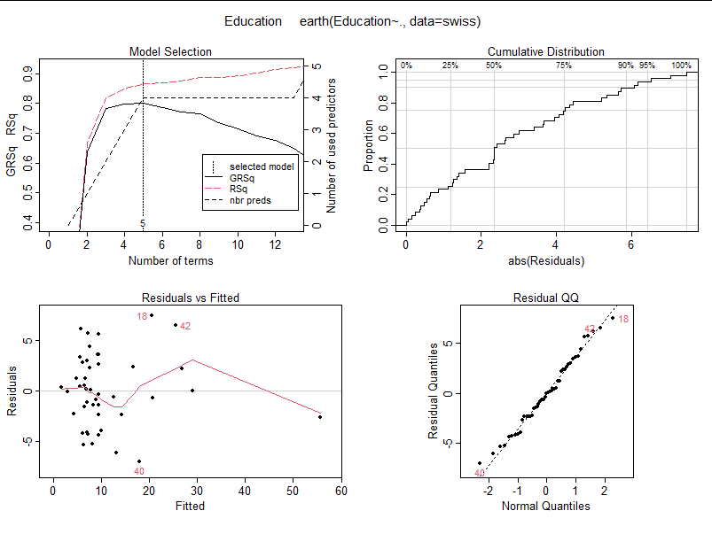
1. Machine learning -- regression analysis
(1) The data were analyzed using earth and caret toolkits
For example, regression analysis of Education for all other elements in swiss;
nls.model <- earth(Education~.,data = swiss)
nls.model
plot(nls.model)
(2) Adjust the parameters of the results (training)
Take n-Fold cross validation as an example, use the train function in the caret package:
train(x, y, method = "rf", preProcess = NULL, ...,
	weights = NULL, metric = ifelse(is.factor(y), "Accuracy",  "RMSE"),
	maximize = ifelse(metric %in% c("RMSE", "logLoss", "MAE"), FALSE, TRUE),
   trControl = trainControl(), tuneGrid = NULL,
   tuneLength = ifelse(trControl$method == "none", 1, 3))
Of which:
x: Input independent variable during fitting
y: Dependent variable input during fitting
Weights: the weights set according to the model are unnecessary
trControl: you need to call the result returned from trainControl() to design an appropriate inspection method
tuneGrid: the method applied in parameter adjustment. Different methods have different parameter adjustment methods, so the column names of the input grid are also different (the function controls parameter adjustment by identifying the column names of the input columns)
For example, a fitting function is established for the Fertility of swiss, and the dependent variable is all other columns:
grid <- expand.grid(
  degree = 1:3,
  nprune = seq(2, 100, length.out = 8)
)
##For a parameter adjustment grid specially constructed by method, degree represents the iteration depth and nprune represents the feature selection quantity
##expand. The grid function will adaptively generate the grid according to rows and columns to meet the matching relationship between data


set.seed(12222)##Generating random seeds ensures the repeatability of the model

swiss.model1 <- train(
x = subset(swiss, select = -Fertility),
y = swiss$Fertility,
method = "earth",
metric = "RMSE",
trControl = trainControl(method = "cv", number = 10),  ## 10% off cross validation
tuneGrid = grid
)
result:
> grid
   degree nprune
1       1      2
2       2      2
3       3      2
4       1     16
5       2     16
6       3     16
7       1     30
8       2     30
9       3     30
10      1     44
11      2     44
12      3     44
13      1     58
14      2     58
15      3     58
16      1     72
17      2     72
18      3     72
19      1     86
20      2     86
21      3     86
22      1    100
23      2    100
24      3    100
> swiss.model1
Multivariate Adaptive Regression Spline

47 samples
 5 predictor

No pre-processing
Resampling: Cross-Validated (10 fold)
Summary of sample sizes: 42, 42, 42, 42, 42, 44, ...
Resampling results across tuning parameters:

  degree  nprune  RMSE       Rsquared   MAE
  1         2     11.278358  0.3284905  9.209832
  1        16      9.541177  0.5068536  7.839405
  1        30      9.541177  0.5068536  7.839405
  1        44      9.541177  0.5068536  7.839405
  1        58      9.541177  0.5068536  7.839405
  1        72      9.541177  0.5068536  7.839405
  1        86      9.541177  0.5068536  7.839405
  1       100      9.541177  0.5068536  7.839405
  2         2     11.294113  0.3270052  9.216748
  2        16     10.717470  0.4382987  8.802805
  2        30     10.717470  0.4382987  8.802805
  2        44     10.717470  0.4382987  8.802805
  2        58     10.717470  0.4382987  8.802805
  2        72     10.717470  0.4382987  8.802805
  2        86     10.717470  0.4382987  8.802805
  2       100     10.717470  0.4382987  8.802805
  3         2     11.294113  0.3270052  9.216748
  3        16     10.798077  0.4366048  8.891187
  3        30     10.798077  0.4366048  8.891187
  3        44     10.798077  0.4366048  8.891187
  3        58     10.798077  0.4366048  8.891187
  3        72     10.798077  0.4366048  8.891187
  3        86     10.798077  0.4366048  8.891187
  3       100     10.798077  0.4366048  8.891187

RMSE was used to select the optimal model using the smallest value.
The final values used for the model were nprune = 16 and degree = 1.
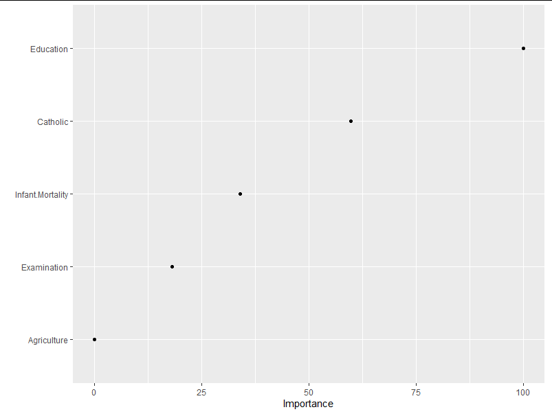
(3) vip is used to show the importance of different independent variables in the result model
library(vip);
p1 <- vip(swiss.model1, num_features = 4, geom = "point", value = "gcv")
Where num_features controls the number of variables to be displayed (priority is given to those with significant influence). value is an indicator of quantitative importance, "gcv" means "Generalized cross − validation". You can also enter "rss" to measure importance by Residual Sums of Squares.
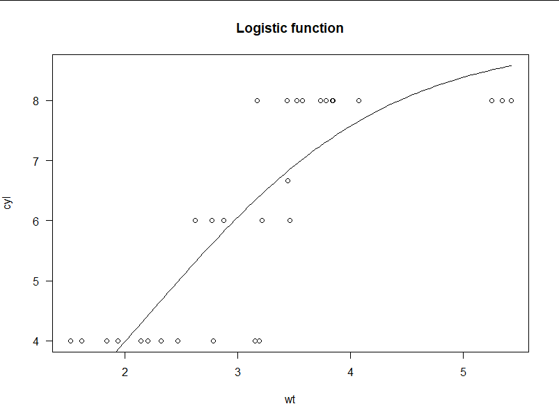
2. Logistic regression
> m <- drm(cyl ~ wt, fct = L.3(), data = mtcars)
> plot(m, log="", main = "Logistic function")

##For example, natural data do not fit the logistic regression curve
3. Nonlinear least square method
(1) Use nls function
nls(formula, data, start, control, algorithm,
    trace, subset, weights, na.action, model,
    lower, upper, ...)
Formula: the formula needs to know the regression model in advance, and the function is only to fit the appropriate parameters
start: it can be a list that records the initial values of various parameters in a model function that cannot be started by itself
Control: a control of fitting conditions
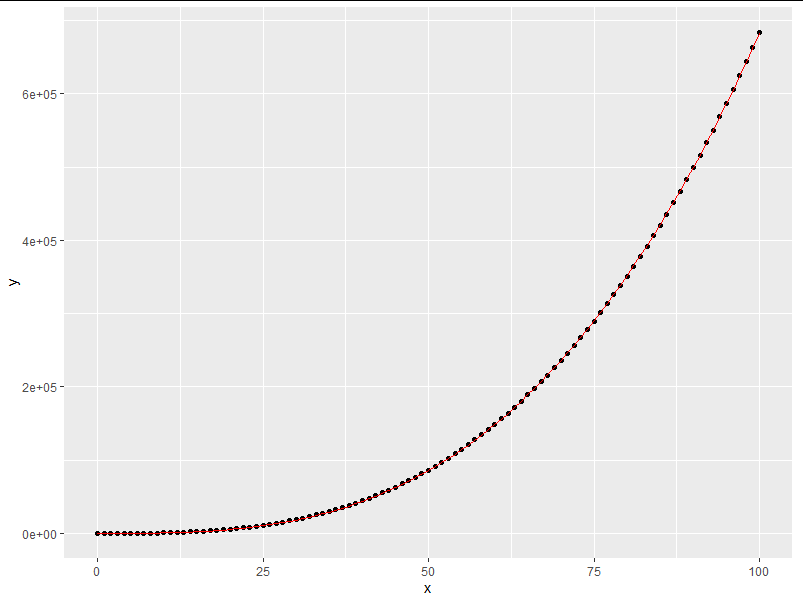
set.seed(43247)
x<-seq(0, 100, 1)
y<-(rnorm(1,0,1)*x^2+runif(1,0,1)*x^3 +rnorm(101,0,1))
m<-nls(y~(a*x^2+b*x^3),
       control = nls.control(maxiter = 100000),  ##Control the maximum number of iterations
       start = list(a=1, b=1));
result:
> m
Nonlinear regression model
  model: y ~ (a * x^2 + b * x^3)
   data: parent.frame()
      a       b
-0.7908  0.3721
 residual sum-of-squares: 87.8

Number of iterations to convergence: 1
Achieved convergence tolerance: 5.332e-09
(2) Automatic fitting using drm function
There is no need to know the function form in advance, only select the model with input, and adaptively start the fitting
library(drc)
m <- drm( y ~ x, fct = LL.3() ); ## Built in model
dat = data.frame(x=x,y=y,nls=predict(m)) ##When predict only inputs the model, it is equivalent to getting a function file
ggplot( dat,aes(x=x,y=y) ) +
  geom_point() + geom_line( aes(x = x, y = nls), colour = "red");

'''
##fct: a list with three or more elements specifying the non-linear function, the accompanying self starter function, the names of the parameter in the non-linear function and, optionally, the first and second derivatives as well as information used for calculation of ED values. Currently available functions include, among others, the four- and five-parameter log-logistic models LL.4, LL.5 and the Weibull model W1.4. Use getMeanFunctions for a full list.

LL.3:

LL.3(fixed = c(NA, NA, NA), names = c("b", "d", "e"), ...)

f(x) = 0 + \frac{d-0}{1+\exp(b(\log(x)-\log(e)))}
'''