R, Redundancy Analysis (RDA), ggplot2

_In the field of ecological environment, redundancy analysis (RDA) is a commonly used analysis method to analyze the impact of "explanatory variables" on "response variables".There are also CCA methods similar to RDA.Here take RDA as an example_After data processing and analysis, we need to visualize the results. The R language ggplt2 package is undoubtedly a visual artifact. However, how to use ggplot2 to visualize RDA results requires us to understand the RDA results and extract the elements that need to be displayed.

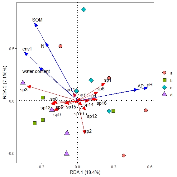
 library(vegan)
  library(ggplot2)
  library(ggrepel)
  fc=read.csv("D:\\wyktang\\factor.csv",header = T,row.names = 1)#Reading explanatory variable data
  sp=read.csv("D:\\wyktang\\sp.csv",header = T,row.names = 1)#Read response variable data
  spp=decostand(sp,method = "hellinger")#Convert response variables
  fcc=log10(fc)#Converting explanatory variables
  uu=rda(spp~.,fcc)#RDA Analysis
ii=summary(uu)  #View analysis results
sp=as.data.frame(ii$species[,1:2])*2#Depending on the drawing result, the drawing data can be enlarged or reduced to a certain extent, as follows
st=as.data.frame(ii$sites[,1:2])
yz=as.data.frame(ii$biplot[,1:2])
grp=as.data.frame(c(rep("a",4),rep("b",4),rep("c",4),rep("d",4)))#Grouping by Square Type
colnames(grp)="group"
 ggplot() +
   #geom_text_repel(data = st,aes(RDA1,RDA2,label=row.names(st)),size=4)+#Show a Square
   geom_point(data = st,aes(RDA1,RDA2,shape=grp$group,fill=grp$group),size=4)+
   scale_shape_manual(values = c(21:25))+
    geom_segment(data = sp,aes(x = 0, y = 0, xend = RDA1, yend = RDA2), 
                 arrow = arrow(angle=22.5,length = unit(0.35,"cm"),
                               type = "closed"),linetype=1, size=0.6,colour = "red")+
        geom_text_repel(data = sp,aes(RDA1,RDA2,label=row.names(sp)))+
   geom_segment(data = yz,aes(x = 0, y = 0, xend = RDA1, yend = RDA2), 
                arrow = arrow(angle=22.5,length = unit(0.35,"cm"),
                              type = "closed"),linetype=1, size=0.6,colour = "blue")+
   geom_text_repel(data = yz,aes(RDA1,RDA2,label=row.names(yz)))+
         labs(x=paste("RDA 1 (", format(100 *ii$cont[[1]][2,1], digits=4), "%)", sep=""),
              y=paste("RDA 2 (", format(100 *ii$cont[[1]][2,2], digits=4), "%)", sep=""))+
          geom_hline(yintercept=0,linetype=3,size=1) + 
            geom_vline(xintercept=0,linetype=3,size=1)+
   guides(shape=guide_legend(title=NULL,color="black"),
          fill=guide_legend(title=NULL))+
              theme_bw()+theme(panel.grid=element_blank())

• 

  _RDA has been explored, but of course, this is just a simple example. Before doing constrained sorting analysis, we need to check whether the data conforms to RDA or CCA. There are many examples on the Internet, which will not be repeated here.When RDA or CCA can't solve our problem well, we need to combine other analysis methods, such as gbm, RF to find relative importance, etc. and also use SEM to explore.In principle, different data needs to be explored in different ways, choose the best result, we cannot blindly model others'methods, we need to depend on our own data analysis results.
  _Friends who have just met R may choose easier CANOCO software because of its "difficult" entry. Of course, the latter is also the data analysis artifact in the field of ecological environment. However, when we want to personalize the analysis and mapping, the latter cannot be satisfied at present. R should be the first choice.To speed up the speed of data analysis and drawing for beginners, we have created a QQ group: 335774366.Welcome interested friends to join guide.
  Disclaimer: The above content is only for the author's personal understanding, there are some errors, you are welcome to correct.