Random forest
1.1 overview of integration algorithm
Integrated learning(
ensemble learning
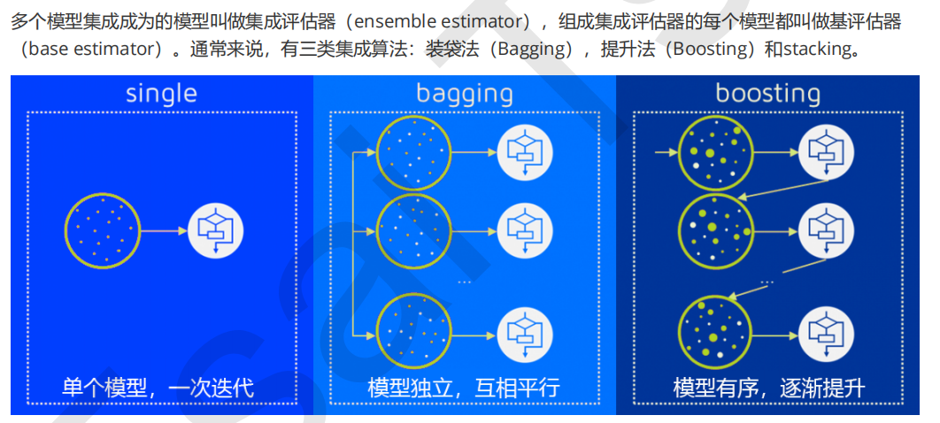
)It is a very popular machine learning algorithm. It is not a single machine learning algorithm, but integrates the modeling results of all models by building multiple models on the data. Basically, integrated learning can be seen in all machine learning fields. In reality, integrated learning also plays a considerable role. It can be used to model marketing simulation, count customer sources, retention and loss, and predict disease risk and patient susceptibility. In the current various algorithm competitions, random forest, gradient lifting tree (GBDT), Xgboost
And other integration algorithms can also be seen everywhere, which shows their good effect and wide application.


1.2 integration algorithm in sklearn
More than half of the integration algorithms are tree integration models. It can be imagined that the decision tree must have a good effect in the integration. In this class, we will take random forest as an example to slowly uncover the mystery of integration algorithm.
This is the number of trees in the forest, that is, the number of base evaluators. The influence of this parameter on the accuracy of the random forest model is monotonic,
n_estimators
More
Large, the effect of the model is often better
. But correspondingly, any model has a decision boundary,
n_estimators
After reaching a certain degree, the accuracy of random forest often does not rise or begin to fluctuate, and n_estimators
The larger the, the larger the amount of computation and memory required, and the longer the training time will be. For this parameter, we are eager to strike a balance between training difficulty and model effect.
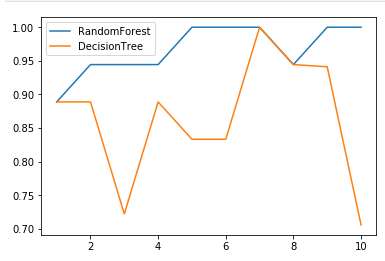
Compare random forest and decision tree
labels="RandomForest"
for i in [RandomForestClassifier(n_estimators=25),DecisionTreeClassifier()]:
    score=cross_val_score(i,X,y,cv=10)
    plt.plot(range(1,11),score,label=labels)
    labels="DecisonTree"
plt.legend()
plt.show()


from sklean.ensemble import RandomForestClassifier as RFC
rfc=RFC(n_estimators=25,random_state=0)
rfc=fit(X,y)
rfc.estimators_#The representative views the information of each tree.
rfc.estimators_[0].random_state#View the random of the first tree_ State attribute
 To view all trees random_state Cycle must be used and cannot be used DataFrame call out random_state
for i in range(len(rfc.estimators_)):
    print(rfc.estimators_[i].random_state)

2.1.4 bootstrap & oob_score
Random forest can not be divided into training set and test set.


If you want to test with out of pocket data, you need to set it when instantiating
oob_score
This parameter is adjusted to
True
, after training, we can use
Another important attribute of random forest:
oob_score_
To view our test results on out of pocket data:
Partition dataset
from sklearn.datasets import load_wine
from sklearn.model_selection import train_test_split
Xtrain,Xtest,Ytrain,Ytest=train_test_split(wine.data,wine.target,test_size=0.3)
rfc=RandomForestClassifier(random_state=20)
rfc=rfc.fit(Xtrain,Ytrain)
score_r=rfc.score(Xtest,Ytest)
Do not divide data sets
rfc=RandomForestClassifier(n_estimators=25,oob_score=True)
rfc=rfc.fit(wine.data,wine.target)
rfc.oob_score_#Returns the score of the out of pocket test

rfc = RandomForestClassifier(n_estimators=25)
rfc = rfc.fit(Xtrain, Ytrain)
rfc.score(Xtest,Ytest)
rfc.feature_importances_
rfc.apply(Xtest)
rfc.predict(Xtest)
rfc.predict_proba(Xtest)#Probability of label assigned to each sample
#There is no predict to return to the forest_ For the interface of proba, because the regressions are all continuous labels, there is no probability of classification
RandomForestRegressor
In the regression tree,
MSE
It is not only our branch quality measure, but also our most commonly used balance
Quantitative regression tree is an index of regression quality
However,
Interface of regression tree
score
Returned is
R
Square, not
MSE
.

from sklearn.ensemble import RandomForestRegressor
from sklearn.model_selection import cross_val_score
rfc=RandomForestRegressor(n_estimators=25)
score=cross_val_score(rfc,X,y,cv=10,scoring="neg_mean_squared_error")
#sklearn is an indicator of all model properties
import sklearn
sorted(sklearn.metrics.SCORERS.keys())
Filling missing values with regression forest
The data we collect from reality can hardly be perfect, and there are often some missing values. In the face of missing values, many people choose to delete the samples containing missing values directly, which is an effective method, but sometimes filling the missing values will be better than directly discarding the samples, even if we don't know the real appearance of the missing values. In sklearn, we can use sklearn. Impulse. Simpleimputer to easily fill the mean, median and other values into the data.
Use sklearn.impulse.simpleimputer to fill in the missing values
Let's fill in the missing value first. Suppose we need 50% of the missing value
import numpy as np
import pandas as pd
from sklearn.datasets import load_boston
from sklearn.impute import SimpleImputer
boston=load_boston()
X_full=boston.data
y_full=boston.target()
missing__rate=0.5
#Add missing values based on index
n_samples=X_full.shape[0]
n_features=y_full.shape[1]
rng=np.random.RandomState(0)
n_missing_samples=int(np.floor(n_samples*n_feature*missing_rate))
#np.floor rounds down and returns a floating-point number in. 0 format
missing_samples=rng.randint(0,n_samples,n_missing_samlpes)
missing_features=rng.randint(0,n_features,n_missing_samples)
X_missing=X_full.copy()
y_missing=y_full.copy()
X_missing[missing_samples,missing_features]=np.nan
X_missing=pd.DataFrame(X_missing)
Fill in missing values with zeros and means
#Filling with mean
from sklearn.impute import SimpleImputer
imp_mean=SimpleImputer(missing_values=np.nan,strategy='mean')
X_missing_mean=imp_mean.fit_transform(X_missing)
#Fill with 0
from sklearn.impute import SimpleImputer
imp_0=SimpleImputer(missing_values=np.nan,strategy="constant",fill_value=0)
X_missing_0=imp_0.fit_transform(X_missing)
Fill with random forest
X_missing_reg=X_missing.copy()
Find the columns with missing values and sort them from small to large,sort The function returns a value from small to large, argsort Returns the index corresponding to the value, from small to large
sortindex=np.argsort(X_missing_reg.isnull().sum()).values
for i in sortindex:
    #Building a new matrix
    df=X_missing_reg
    fillc=df.iloc[:,i]
    df=pd.concat([df.iloc[:,df.columns!=i],pd.DataFrame(y_missing)],axis=1)

    df_0=SimpleImputer(missing_values=np.nan,strategy="constant",fill_value=0)
    df_0=df_0.fit_transform(df)

    Find out the training set and test set
    Ytrain=fillc[fillc.notnull()]
    Ytest=fillc[fillc.isnull()]
    Xtrain=df_0[Ytrain.index,:]
    Xtest=df_0[Ytest.index,:]

    rfc=RandomForestRegressor(n_estimators=25).fit(Xtrain,Ytrain)
    Ypredict=rfc.predict(Xtest,Ytest)
    X_missing_reg.iloc[X_missing_reg.iloc[:,i].isnull(),i]=Ypredict
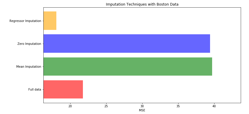
Compare the scores of original data set, 0 and mean filling data set and regression forest filling data set
X=[X_full,X_missing_mean,X_missing_0,X_missing_reg]
mse=[]
for i in X:
    reg=RandomForestRegressor(n_estimators=100,random_state=1)
    score=cross_val_score(reg,i,y_full,scoring="neg_mean_squared_error",cv=5).mean()
    mse.append(score*-1)
[*zip(["X_full","X_missing_mean","X_missing_0","X_missing_reg"],mse)]


x_labels=['Full data'
          ,'Mean Imputation'
          ,'Zero Imputation'
          ,'Regressor Imputation'
]
colors=['r','g','b','orange']
plt.figure(figsize=(12,6))
ax=plt.subplot(111)
for i in range(len(mse)):
    ax.barh(i,mse[i],color=colors[i],alpha=0.6,align='center')
    #In barh, h represents transverse and alpha represents columnar coarseness
ax.set_title('Imputation Techniques with Boston Data')
ax.set_xlim(left=np.min(mse)*0.9,right=np.max(mse)*1.1)
ax.set_yticks(range(len(mse)))
ax.set_xlabel('MSE')
ax.set_yticklabels(x_labels)
plt.show()
