Reading Notes: Chapter 7 Convolutional Neural Network

The topic of this chapter is Convolutional Neural Network (CNN). CNN is used in image recognition, speech recognition and other situations. In image recognition competitions, depth-based learning methods are almost based on CNN.

7.1 Overall Structure

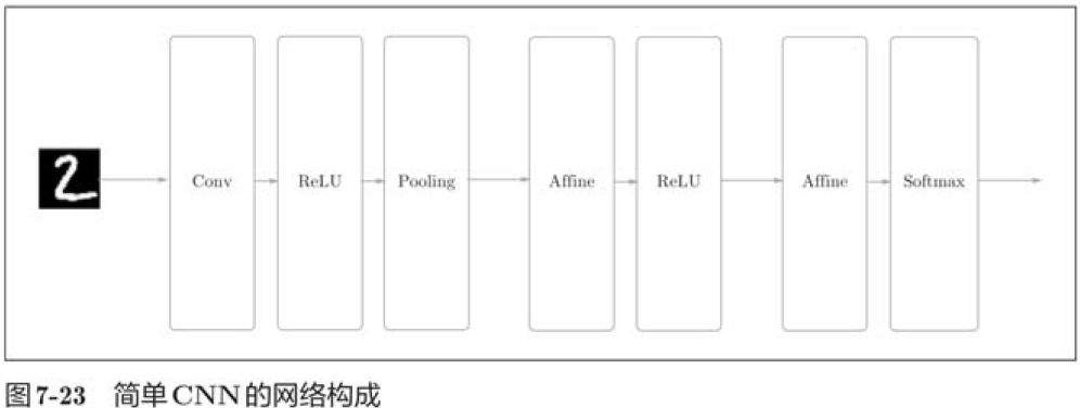
Like the neural networks described earlier, CNNs can be built from assembly layers just like Lego blocks. However, convolution and pooling layers occur in CNNs.

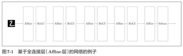
In the previously described neural network, all the neurons in the adjacent layers have connections, which are called full connections. In addition, we implemented a full connection layer with the Affine layer.

So what kind of structure would CNN be?

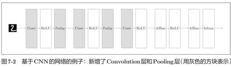In the figure above, the previous Affine-ReLU combination is used in layers near the output, and the previous Affine-Softmax combination is used in the final output layer. These are common structures in general CNN s.

7.2 Convolution Layer

There are some unique terms in CNN, such as padding, pacing, etc. In addition, the data transferred in each layer is shaped, which is different from previous fully connected networks.

Problems with 7.2.1 Full Connection Layer

What's wrong with the full connection layer? The shape of the data is ignored. For example, when the input data is an image, the image is usually a three-dimensional shape in the direction of height, length, and channel. However, when entering into the full connection layer, the three-dimensional data needs to be flattened to one-dimensional data.

Images are three-dimensional and should contain important spatial information. For example, there are similar values for adjacent pixels in space, close correlations between channels of RGB, no correlations among distant pixels, etc. There may be intrinsic patterns that are worth extracting hidden in 3-D shapes, but because the full connectivity layer ignores the shape, all input data is processed as the same neuron (the same dimension neuron). So you can't take advantage of shape-related information.

The convolution layer can keep its shape unchanged. When the input data is an image, the convolution layer receives the input data as three-dimensional data and outputs it to the next layer as three-dimensional data. Therefore, in a CNN, it is possible to correctly understand data with shapes, such as images.

In addition, the input and output data of convolution layers are sometimes referred to as feature maps in CNN s. The input data of the convolution layer is called the input characteristic map, and the output data is called the output characteristic map.

7.2.2 Convolution

The convolution layer is a convolution operation, which is equivalent to the "filter operation" in image processing.

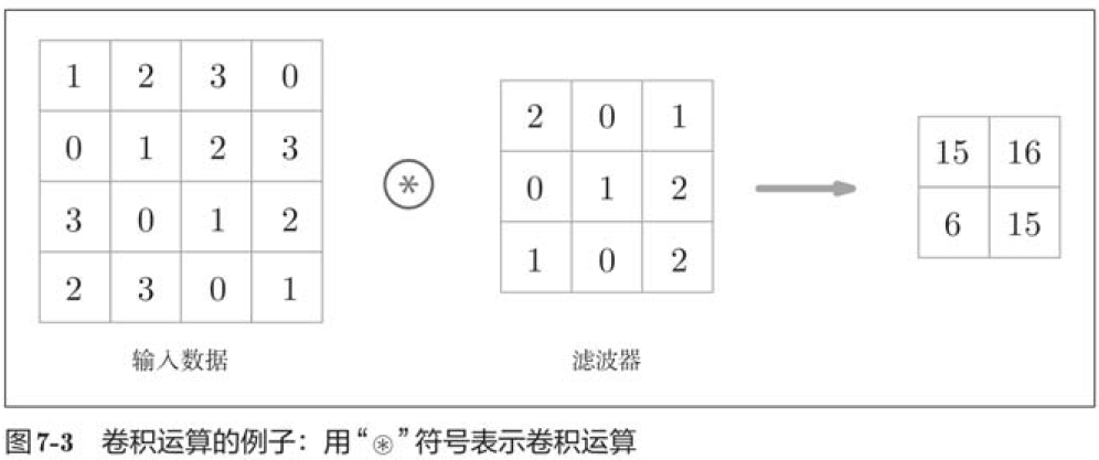
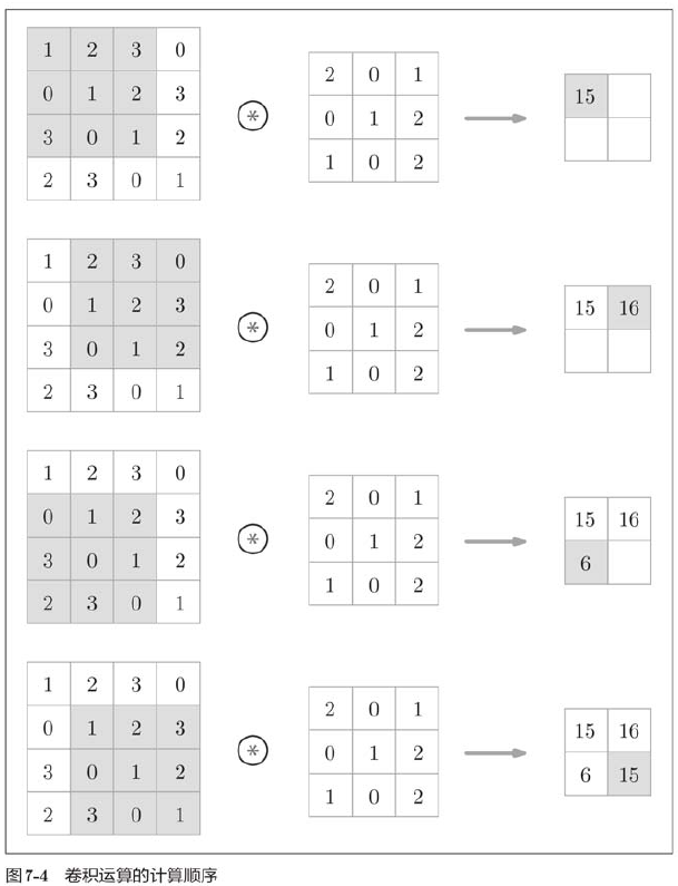
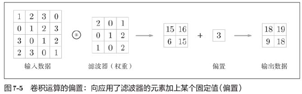
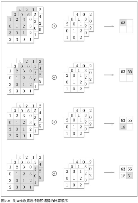
For input data, the convolution operation is applied with a sliding filter window at a certain interval. As shown in the figure, the elements of the filter at each location are multiplied by the corresponding elements of the input, and then summed (sometimes referred to as multiplication, accumulation, and addition). This result is then saved to the corresponding location of the output, and the output of the convolution operation can be obtained by repeating the process in all locations.

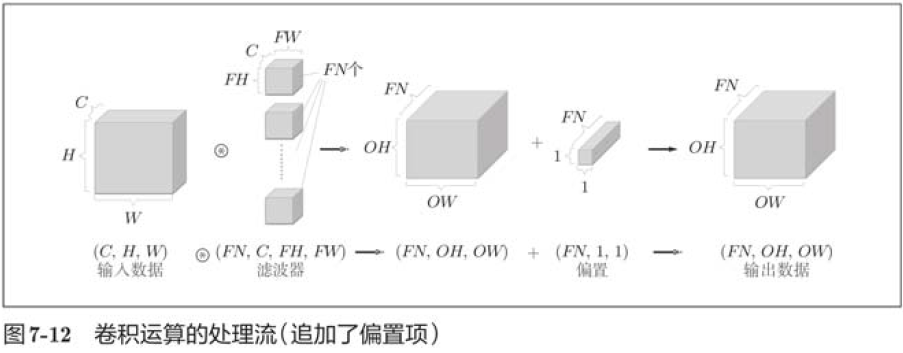
In fully connected neural networks, there are biases in addition to the weight parameters. In a CNN, the parameters of the filter correspond to the previous weights, and there is a bias in the CNN.

7.2.3 Fill

Before processing convolution layers, it is sometimes necessary to fill fixed data (such as 0) around the input data, which is called filling and is often used in convolution operations.

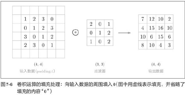
Filling is used primarily to resize the output. For example, when a filter (3,3) is applied to input data of size (4,4), the output size becomes (2,2), which is equivalent to two elements smaller than the input size. This can become a problem in deep networks where multiple convolutions are repeated. Why? Because each convolution operation reduces space, it is possible that at some point the output size will become 1, making the convolution impossible to apply. To avoid this, use padding. In the previous example, set the fill to 1, and the output size will remain the same as the input size (4,4). Therefore, convolution allows data to be passed down to the next level while maintaining the same size of space.

7.2.4 steps

The position interval at which the filter is applied is called the step.

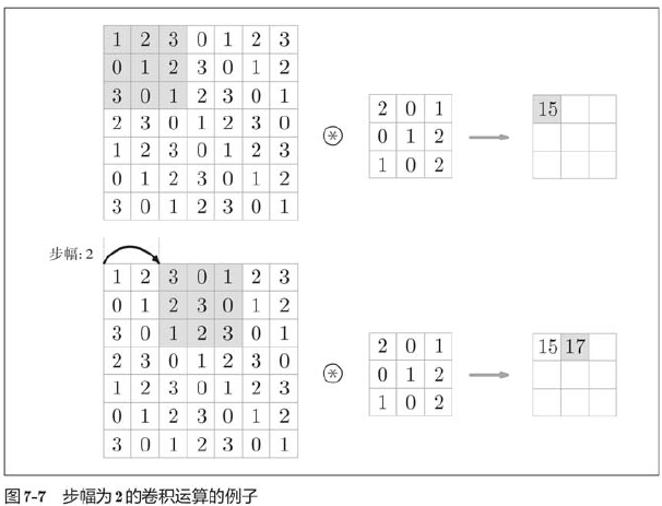
Increasing the step size decreases the output size, while increasing the fill size increases the output size.

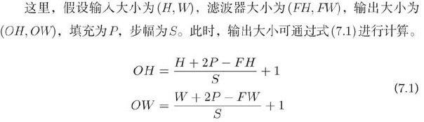
When the output size is not divisible (the result is a decimal), measures such as errors need to be taken. By the way, depending on the framework of in-depth learning, when the value cannot be divided, it sometimes rounds to the nearest integer and continues without error.

Convolution of 7.2.5 3-D data

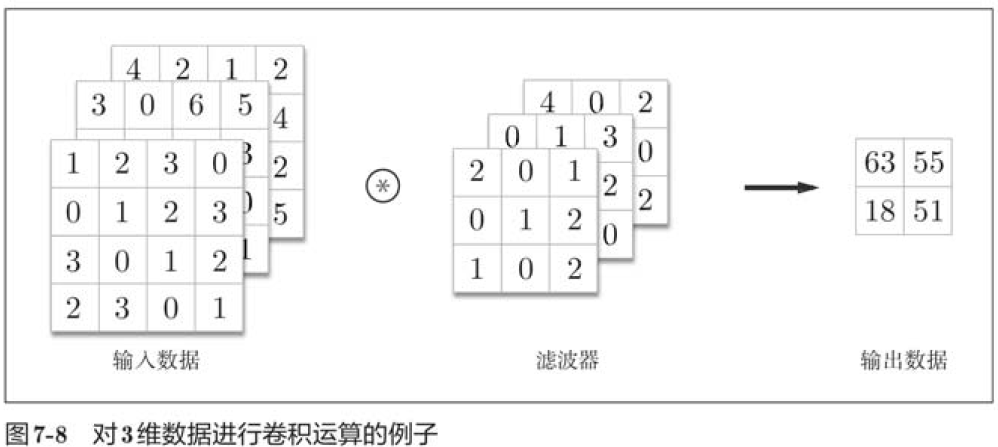
When there are multiple signatures along the channel direction, the convolution of the input data and the filter is performed by the channel, and the results are added together to obtain the output. (

In convolution of 3-D data, the number of channels of the input data and the filter should be set to the same value, and the filter size can be set to any value.

7.2.6 Combining Block Thinking

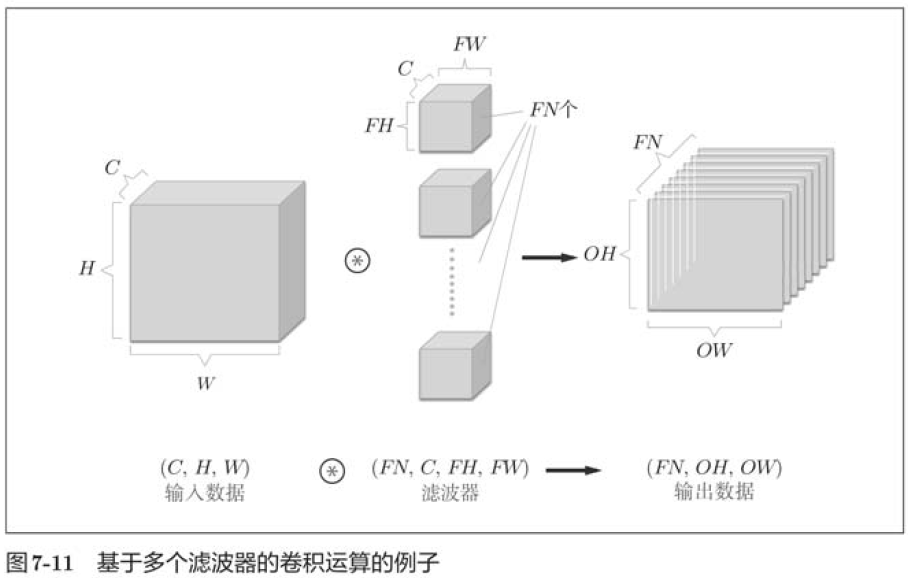
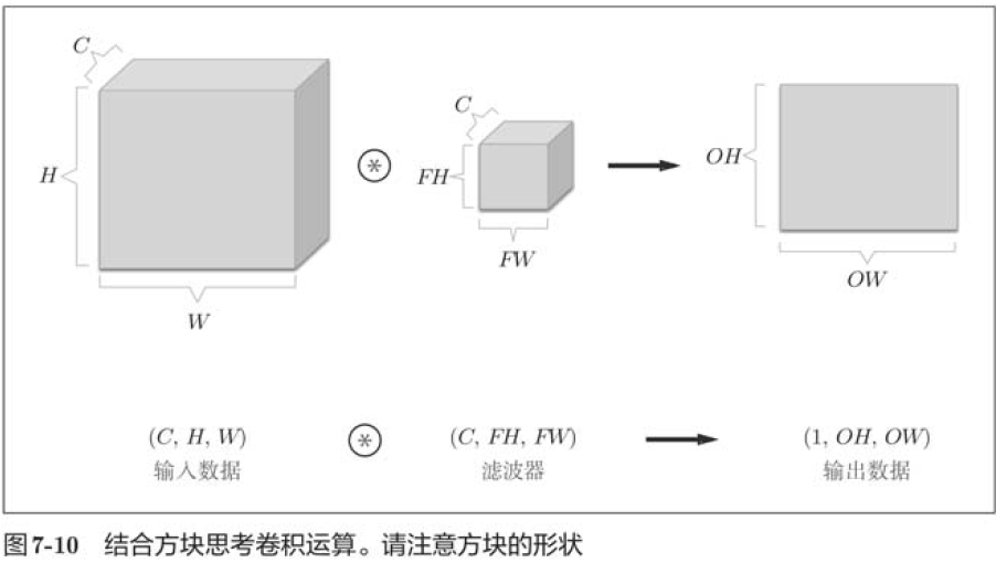In this example, the data output is a signature graph. The so-called 1 feature map, in other words, is a feature map with 1 channel number. So what if you want to have multiple convolution outputs in the channel direction as well? To do this, multiple filters (weights) are needed.

7.2.7 Batch Processing

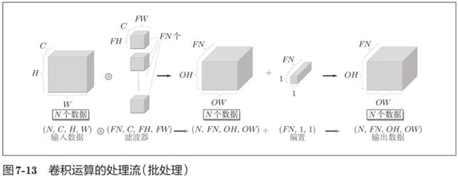
Batch processing is used to package input data in the processing of the neural network. Previous implementation of the fully connected neural network also corresponds to batch processing, which enables efficient processing and mini-batch correspondence in learning.

We want convolution to correspond to batch processing as well, so we need to save the data passed between layers to 4-dimensional data. Specifically, the data is saved in batch_num, channel, height, width order.

7.3 Pooling Layer

Pooling is the operation of reducing space in both high and long directions.

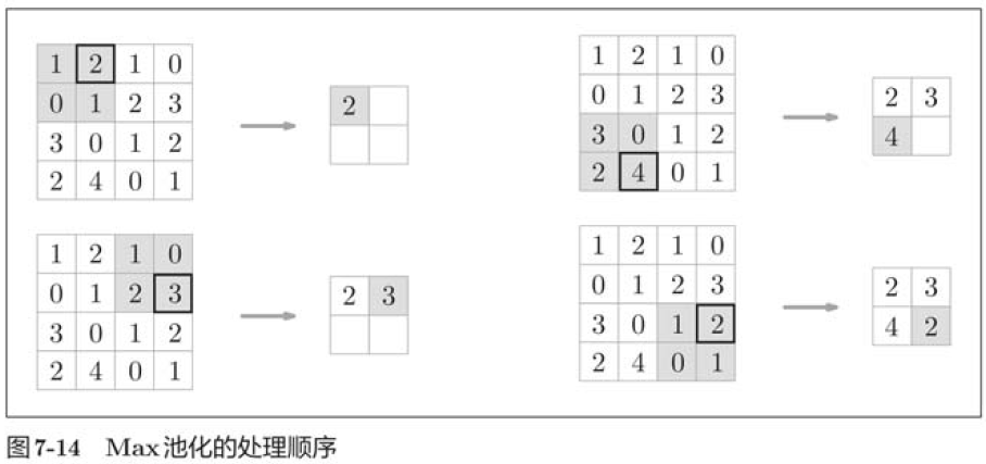
"Max pooling" is an operation to get the maximum value, and "2x2" represents the size of the target area. Generally speaking, the pooled serial port size is set to the same value as the step size.

In addition to Max pooling, there are Average pooling, and so on. Relative to Max pooling, Average pooling calculates the average value of the target area. In the field of image recognition, Max pooling is mainly used. So when we talk about the "pooled layer" in this book, we mean Max pooling.

Characteristics of the pooled layer

1. There are no parameters to learn.

The pooling and convolution layers are different and have no parameters to learn. Pooling simply takes the maximum (or average) value from the target area, so there are no parameters to learn.

2. Number of channels does not change

After pooling, the number of channels for input and output data does not change.

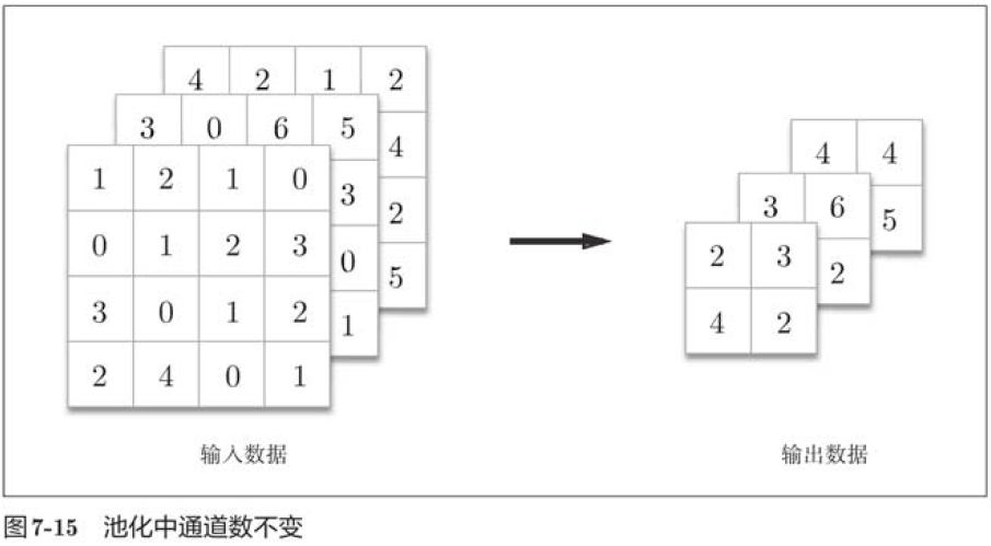
As shown in the figure above, the calculation is done independently by channel.

3. Robustness to small position changes (robustness)

Pooling returns the same result when the input data has a smile bias. Therefore, pooling is robust to small deviations from input data.

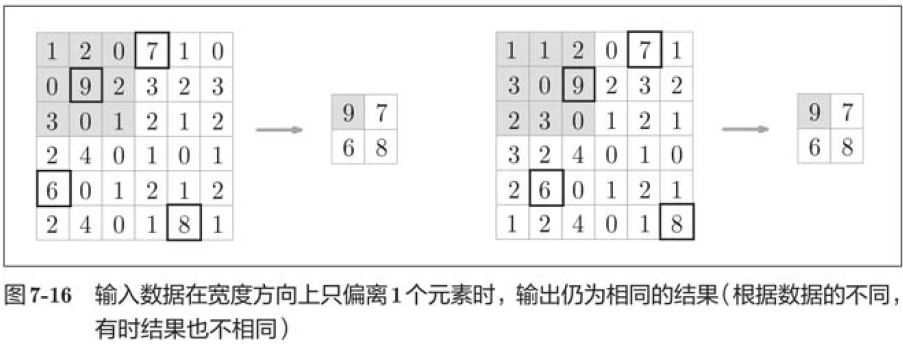
As shown in the figure above, pooling absorbs deviations from the input data (depending on the data, the results may be inconsistent).

7.4 Implementation of Convolution Layer and Pooling Layer

7.4.1 4-dimensional array

import numpy as np
x = np.random.rand(10, 1, 28, 28)
print(x.shape)
print(x[0].shape)
print(x[1].shape)
print(x[0, 0])
print(x[0][0])

(10, 1, 28, 28)
(1, 28, 28)
(1, 28, 28)
[[0.78366725 0.04926278 0.19718404 0.57338282 0.39769665 0.01094044
  0.824495   0.91850354 0.73099492 0.71527378 0.35505084 0.0211244
  0.73428751 0.43283415 0.62773291 0.04168173 0.53651204 0.27816881
  0.16277058 0.49880375 0.26565717 0.03620092 0.71409177 0.40914321
  0.47988124 0.3231364  0.92026101 0.57861158]
 [0.79113883 0.40655301 0.42514531 0.26880885 0.80510278 0.13539557
  0.53198892 0.19315611 0.55525788 0.68411349 0.01468148 0.951923
  0.50952119 0.39191196 0.8592221  0.88079757 0.14027045 0.41493338
  0.3364961  0.21514096 0.81014103 0.4290779  0.84423908 0.5519229
  0.87218471 0.96769902 0.93064515 0.21332042]
......

7.4.2 Expansion based on im2col

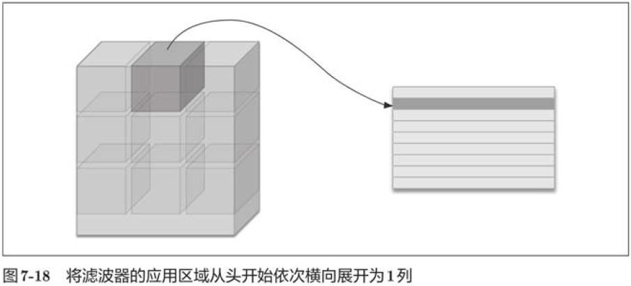
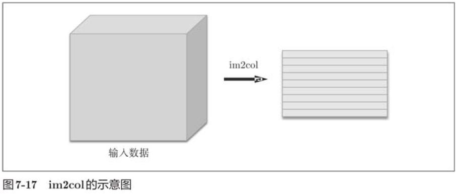Im2col expands the input data to fit the filter (weight). For input data, the area (3-dimensional square) where the filter is applied is expanded horizontally into a column, which im2col does in all places where the filter is applied.

Implementation of 7.4.3 Convolution Layer

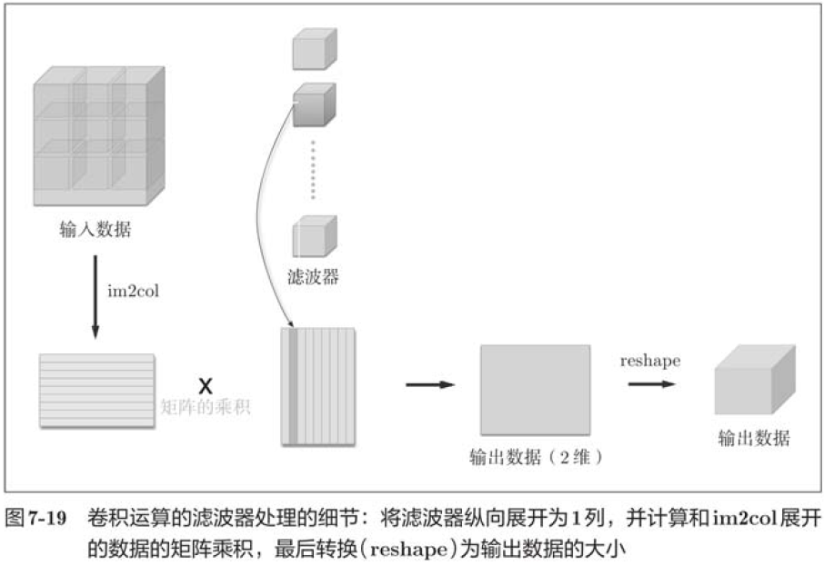
This book provides the im2col function and uses it as a black box (regardless of internal implementation).

im2col expands the input data into a two-dimensional array, taking into account the filter size, step size, and fill.

Now use im2col to implement the convolution layer, where we will implement the convolution layer as a class called Convolution.

class Convolution:
    def __init__(self, W, b, stride=1, pad=0):
        self.W = W
        self.b = b
        self.stride = stride
        self.pad = pad

    def forward(self, x):
        FN, C, FH, FW = self.W.shape
        N, C, H, W = x.shape
        out_h = int(1 + (H + 2*self.pad - FH) / self.stride)
        out_w = int(1 + (W + 2*self.pad - FW) / self.stride)

        col = im2col(x, FH, FW, self.stride, self.pad)
        col_W = self.W.reshape(FN, -1)
        out = np.dot(col, col_W) + self.b

        out = out.reshape(N, out_h, out_w, -1).transpose(0, 3, 1, 2)

        return out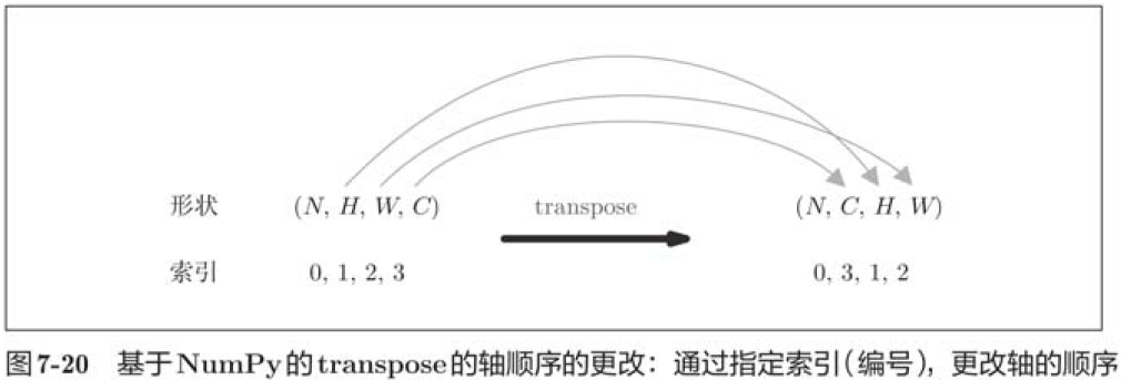

7.4.4 Pooling Layer Implementation

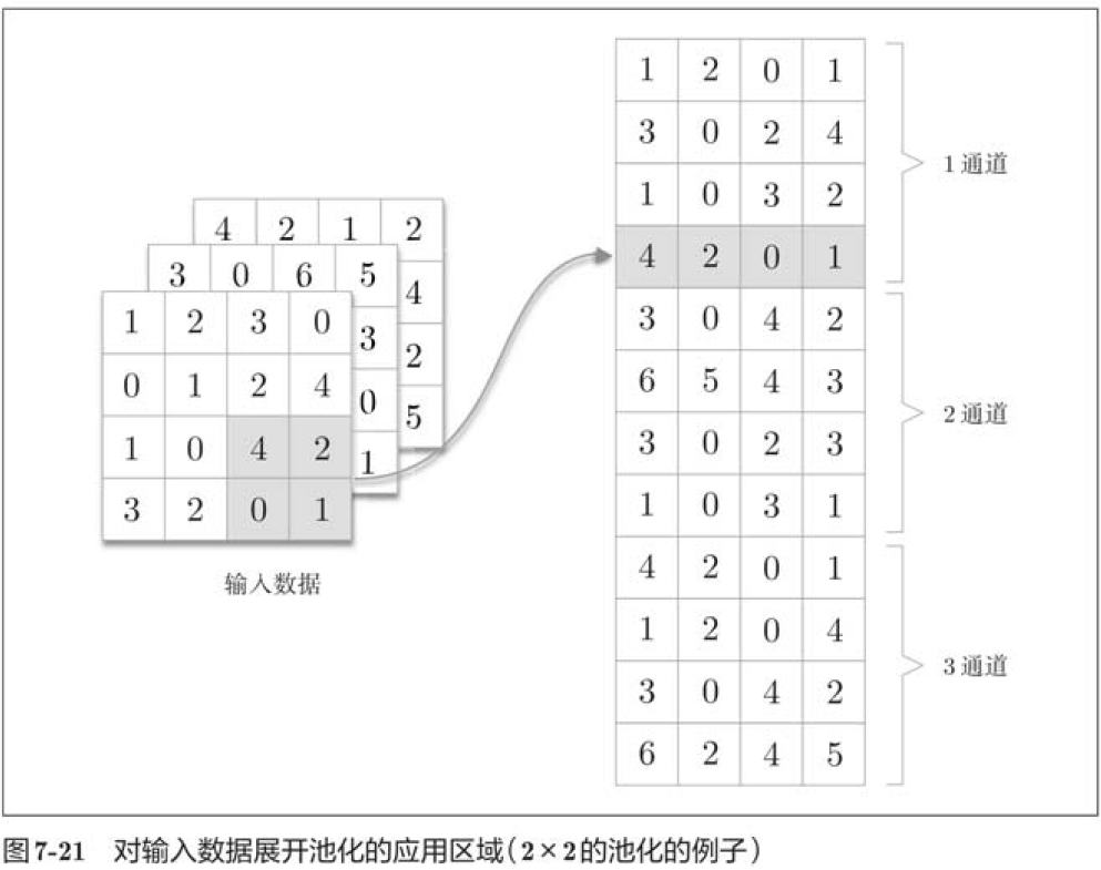
The implementation of the pooling layer is the same as the convolution layer, using im2col to expand the input data. However, in pooled cases, the channel direction is independent, unlike convolution layers. Specifically, pooled application areas are spread out separately by channel.

class Pooling:
    def __init__(self, pool_h, pool_w, stride=1, pad=0):
        self.pool_h = pool_h
        self.pool_w = pool_w
        self.stride = stride
        self.pad = pad

    def forward(self, x):
        N, C, H, W = x.shape
        out_h = int(1 + (H - self.pool_h) / self.stride)
        out_w = int(1 + (W - self.pool_w) / self.stride)

        # Expand (1)
        col = im2col(x, self.pool_h, self.pool_w, self.stride, self.pad)
        col = col.reshape(-1, self.pool_h*self.pool.pool_w)

        # Maximum (2)
        out = np.max(col, axis=1)
        # Conversion (3)
        out = out.reshape(N, out_h, out_w, C).transpose(0, 3, 1, 2)

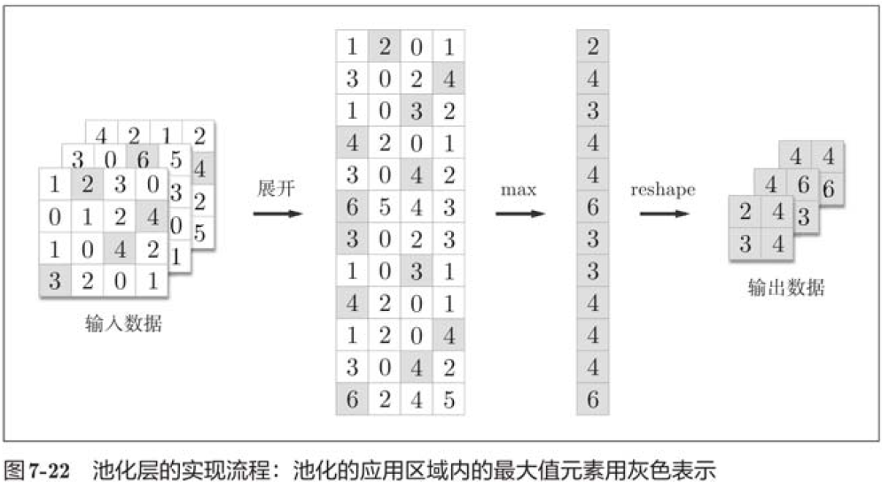
        return out

The pooling layer is implemented in the following three phases:

1. Expand the input data;

2. Maximum value of each row;

3. Convert to the appropriate output size.

Implementation of 7.5 CNN

Now that we have implemented convolution and pooling layers, let's combine them to build CNN s for handwritten number recognition.

class SimpleConvNet:
    def __init__(self, input_dim=(1, 28, 28), conv_param = {'filter_num':30, 'filter_size':5, 'pad':0, 'stride':1}, hidden_size=100, output_size=10, weight_init_std=0.01):
        filter_num = conv_param['filter_num']
        filter_size = conv_param['filter_size']
        filter_pad = conv_param['pad']
        filter_stride = conv_param
        input_size = input_dim[1]
        conv_output_size = (input_size - filter_size + 2*filter_pad) / filter_stride + 1
        pool_output_size = int(filter_num * (conv_output_size/2) * (conv_output_size/2))

        self.params = {}
        self.params['W1'] = weight_init_std * np.random.randn(filter_num, input_dim[0], filter_size, filter_size)
        self.params['b1'] = np.zeros(filter_num)
        self.params['W2'] = weight_init_std * np.random.randn(pool_output_size, hidden_size)
        self.params['b2'] = np.zeros(hidden_size)
        self.params['W3'] = weight_init_std * np.ramdon.randn(hidden_size, output_size)
        self.params['b3'] = np.zeros(output_size)

        self.layers = OrderedDict()
        self.layers['Conv1'] = Convolution(self.params['W1'],
                                           self.params['b1'],
                                           conv_param['stride'],
                                           conv_param['pad'])

        self.layers['Relu1'] = Relu()
        self.layers['Pool1'] = Pooling(pool_h=2, pool_w=2, stride=2)
        self.layers['Affine1'] = Affine(self.params['W2'], self.params['b2'])
        self.layers['Relu2'] = Relu()
        self.layers['Affine2'] = Affine(self.params['W3'], self.params['b3'])
        self.last_layer = SoftmaxWithLoss()

    def predict(self, x):
        for layer in self.layers.values():
            x = layer.forward(x)
        return x

    def loss(self, x, t):
        y = self.predict(x)
        return self.lastLayer.forward(y, t)

    def gradient(self, x, t):
        # forward
        self.loss(x, t)
        
        # backward
        dout = 1
        dout = self.lastLayer.backward(dout)
        
        layers = list(self.layers.values())
        layers.reverse()
        for layer in layers:
            dout = layer.backward(dout)
        
        # Set up
        grads = {}
        grads['W1'] = self.layers['Conv1'].dW
        grads['b1'] = self.layers['Conv1'].db
        grads['W2'] = self.layers['Affine1'].dW
        grads['b2'] = self.layers['Affine1'].db
        grads['W3'] = self.layers['Affine2'].dW
        grads['b3'] = self.layers['Affine2'].db
        
        return grads

Convolution layer and pooling layer are necessary modules in image recognition. CNN can effectively read some characteristics in the image, and can also achieve high-precision recognition in handwritten number recognition.

Visualization of 7.6 CNN

7.6.1 Visualization of Layer 1 Weights

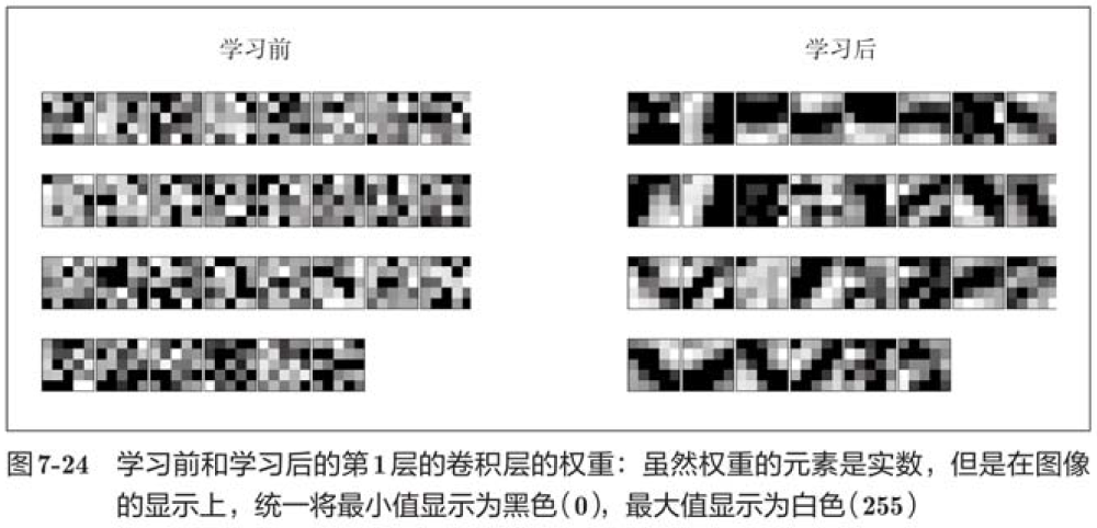
In the figure above, the pre-learning filter is randomly initialized, so there is no regularity in black and white intensity, but the after-learning filter becomes a regular image. We find that by learning, filters are updated to regular filters, such as those with white-to-black gradients, filters with blob s, and so on.

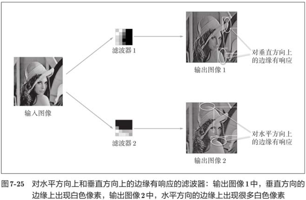
The image above shows the result of convoluting the input image by choosing two learned filters. We find that Filter 1 responds to edges in the vertical direction and Filter 2 responds to edges in the horizontal direction.

Thus, the filter of convolution layer extracts the original information such as edges or patches, and the CNN transmits the original information to the later layer.

7.6.2 Hierarchical Information Extraction

According to visualization-related studies of in-depth learning, as the level of CNN increases, the extracted information (correctly, neurons that reflect a strong response) becomes more and more abstract.

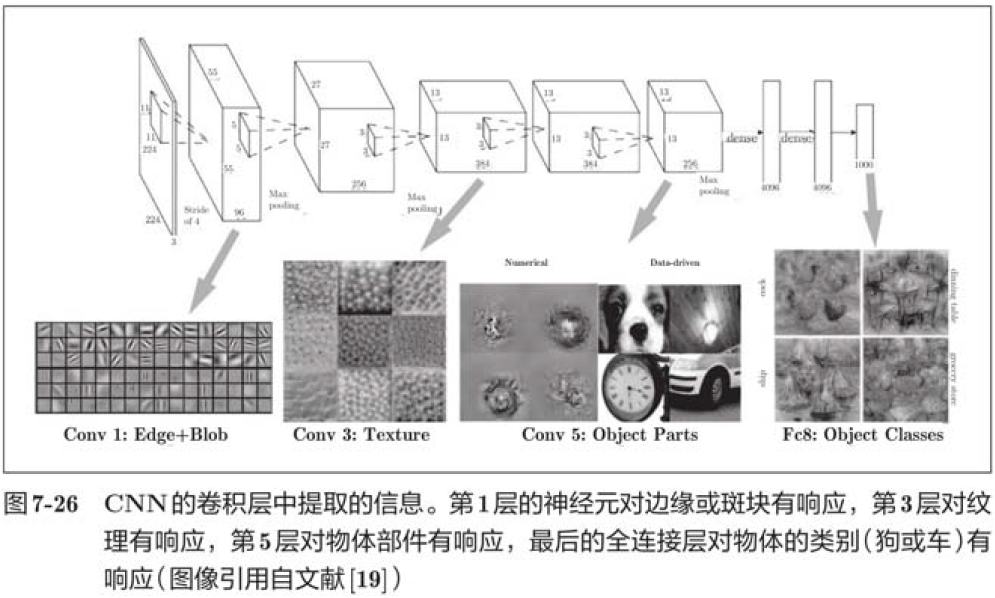As shown in the figure above, if you stack multiple layers of convolution, as the layers get deeper, the extracted information becomes more complex and abstract, which is an interesting place to learn in depth. The first layer responds to simple edges, the next to textures, and the latter to more complex object parts. That is, as the hierarchy increases, neurons change from simple shapes to "advanced" information. In other words, just as we understand what things mean, the objects that respond are gradually changing.

7.7 A representative CNN

7.7.1 LeNet

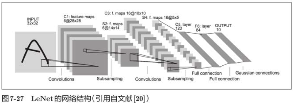
LeNet has continuous convolution and pooling layers (correctly, only a subsampling layer of "selected elements") and outputs the results through the full connection layer.

7.7.2 AlexNet

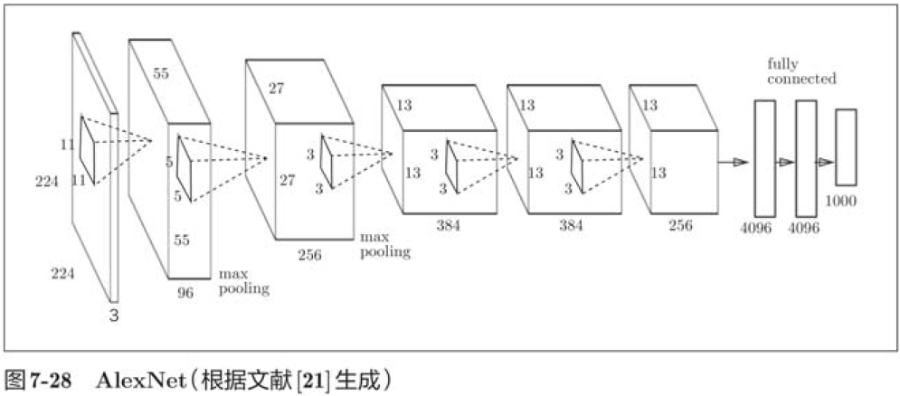
AlexNet stack has multiple convolution and pooling layers and outputs the results through the full connection layer. Although AlexNet and LeNet are not significantly different in structure, there are a few differences:

1. The activation function uses ReLU;

2. Use LRN layers that are locally normalized;

3. Use Dropout.

LexNet is not much different from LexNet in terms of network structure, but there have been great advances in the environment and computer technology around them. Specifically, now anyone can get a lot of data. Moreover, the GPU that is good at large-scale parallel computing has been popularized, and it is possible to do a lot of operations at high speed. Large data and GPU have become a huge driving force for the development of in-depth learning.

In most cases, in-depth learning (a deeper network) has a large number of parameters. Therefore, learning requires a lot of calculation and a lot of data to make those parameters "satisfactory", so it can be said that GPU and big data bring hope to these topics.

7.8 Summary

This chapter describes CNN.

The convolution and pooling layers that make up the basic modules of a CNN are somewhat complex, but once you understand them, you will only be able to use them.

1.CNN adds convolution and pooling layers to the previous fully connected network;

2. Convolution and pooling layers can be easily and efficiently implemented by using im2col function.

3. With the visualization of CNN, we can know that the extracted information becomes more advanced with the deeper level.

4.LeNet and LexNet are representative networks of CNN;

5. In the development of deep learning, big data and GPU have made great contributions.

Topics: Python Deep Learning CNN

Programmer Think