To illustrate the environment, the code is implemented in C + +, but the matrix operation is not implemented in C + +. Making wheels by yourself is a waste of time and unnecessary. Therefore, the Eigen library is used for matrix operation, and the codes of other functions are implemented by yourself.
1, Environment configuration
The Eigen matrix is easy to operate. This paper configures Eigen in the environment of VS2015. The specific Eigen library configuration process will not be described in detail. If you don't know how to configure Eigen, you can see this article https://blog.csdn.net/panpan_jiang1/article/details/79649452 , the environment is like this. The rest of the work is to create a new project and start writing code. This paper uses Eigen3 Version 3.9.
2, Network structure
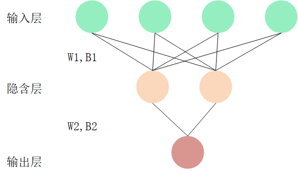
The network has three layers: input layer, hidden layer and output layer. The number of input dimensions of the input layer is 10, the output dimension of the hidden layer is 5 and the output layer is 1. The approximate structure is shown in the figure below:
Come down and go to the specific code part:
The beginning is the fixed parameter part:
#define InputShape 10
#define Layer1_OutShape 5
#define Layer2_OutShape 1
//Data volume
#define DataNum 100
//Number of training rounds
#define Epcho   2000
First, we define the class NN of a neural network. The trainable parameters of a neural network include weight W and threshold B. what is fixed is the learning rate (of course, there is attenuation learning rate, which I didn't do here) and the input value and real (label) value. Therefore, when initializing a neural network, the weight threshold is initialized randomly.
Constructor of NN:
NN::NN(MatrixXf input, MatrixXf y_true, float alph)//Initialization weight
{
	this->input = input;
	this->y_true = y_true;
	this->alph = alph;
	this->W1_T = MatrixXf::Random(Layer1_OutShape, InputShape);
	this->W2_T = MatrixXf::Random(Layer2_OutShape, Layer1_OutShape);
	this->B1 = MatrixXf::Zero(Layer1_OutShape,this->input.cols());
	this->B2 = MatrixXf::Zero(Layer2_OutShape, this->input.cols());
}
Then, establish the forward propagation of the network
MatrixXf NN::ForWard()
{
	this->Z1 = this->W1_T * this->input;
	this->A1 = Leak_ReLu(this->Z1, this->alph);
	this->Z2 = this->W2_T * this->A1;
	this->A2 = Leak_ReLu(this->Z2, this->alph);
	//return MSE(this->y_true, this->A2);
	return this->A2;
}
The mathematical principle of forward propagation is relatively simple,
Input layer to hidden layer:
Z
1
=
W
1
T
∗
i
n
p
u
t
Z_{1}=W_{1}^{T}*input
Z1=W1T∗input,
A 1 = L e a k y _ R e L u ( Z 1 ) A_{1}=Leaky\_ReLu(Z_{1}) A1=Leaky_ReLu(Z1)
L
e
a
k
y
_
R
e
L
u
(
Z
)
=
{
Z
Z
>
=
0
a
l
p
h
∗
Z
Z
<
0
Leaky\_ReLu(Z)=\left\{\begin{matrix} Z & Z>=0 & \\ alph*Z & Z<0 & \end{matrix}\right.
Leaky_ReLu(Z)={Zalph∗ZZ>=0Z<0
The default value of alph is 0.1.
Hidden layer to output layer:
Z
2
=
W
2
T
∗
A
1
Z_{2}=W_{2}^{T}*A_{1}
Z2=W2T∗A1,
A 2 = L e a k y _ R e L u ( Z 2 ) A_{2}=Leaky\_ReLu(Z_{2}) A2=Leaky_ReLu(Z2)
Here comes the play. In the process of back propagation, post the code first^_^
float NN::BackWard()
{
	int rows_temp, cols_temp;//Temporary row column variable
	//Abount Layer2 work start!!
	this->dJ_dA2 = 2 * (this->A2 - this->y_true);
	this->dA2_dZ2 = MatrixXf::Ones(this->Z2.rows(),this->Z2.cols());
	for (rows_temp = 0; rows_temp < this->Z2.rows(); ++rows_temp)
	{
		for (cols_temp = 0; cols_temp < this->Z2.cols(); ++cols_temp)
		{
			this->dA2_dZ2(rows_temp, cols_temp) = this->Z2(rows_temp, cols_temp) >= 0 ? 1.0 : this->alph;
		}
	}
	this->dZ2_dW2 = this->A1.transpose();
	this->dW2 = this->dJ_dA2.cwiseProduct(this->dA2_dZ2)*this->dZ2_dW2/DataNum;
	this->dB2 = this->dJ_dA2.cwiseProduct(this->dA2_dZ2) / DataNum;
	//Abount Layer2 work end!!

	//Abount Layer1 work start!!
	this->dZ2_dA1 = this->W2_T.transpose();
	this->dA1_Z1 = MatrixXf::Ones(this->Z1.rows(), this->Z1.cols());
	for (rows_temp = 0; rows_temp < this->Z1.rows(); ++rows_temp)
	{
		for (cols_temp = 0; cols_temp < this->Z1.cols(); ++cols_temp)
		{
			this->dA1_Z1(rows_temp, cols_temp) = this->Z1(rows_temp, cols_temp) >= 0 ? 1.0 : this->alph;
		}
	}

	this->dZ1_W1 = this->input.transpose();
	this->dW1 = this->dA1_Z1.cwiseProduct(this->dZ2_dA1 * this->dJ_dA2.cwiseProduct(this->dA2_dZ2))*this->dZ1_W1 / DataNum;
	this->dB1 = this->dA1_Z1.cwiseProduct(this->dZ2_dA1 * this->dJ_dA2.cwiseProduct(this->dA2_dZ2)) / DataNum;
	//Abount Layer1 work end!!
	//Adjust learning parameters
	this->W2_T = this->W2_T - this->alph*this->dW2;
	this->W1_T = this->W1_T - this->alph*this->dW1;
	this->B2 = this->B2 - this->alph*this->dB2;
	this->B1 = this->B1 - this->alph*this->dB1;
	return MSE(this->y_true,this->ForWard());
}
Just looking at the code will make you dizzy. Let me explain the whole process first: after NN (neural network) is initialized, feed it with data, and NN will give the predicted value y_pred,y_ PRED must match the real value y_true has error. Use a simple mean square error (MSE) formula according to y_pred and y_true accounting calculates a loss value loss. NN adjusts the weight and threshold according to a certain algorithm based on loss. The goal is to make loss smaller and tend to 0. In this way, y_pred and y_true becomes the same.
OK, how to adjust it? Simply, we think of the gradient descent method. The figure above first
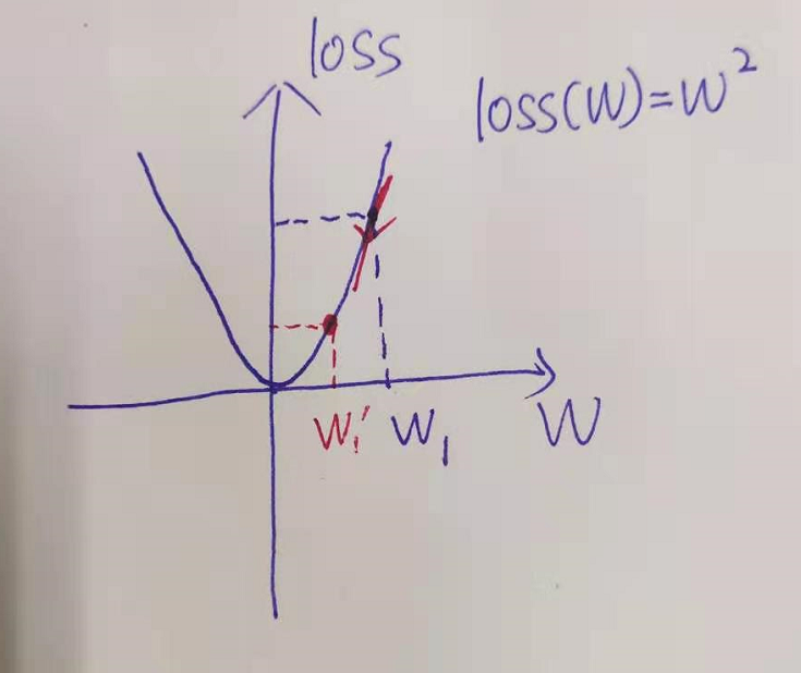
To simplify the problem, our purpose is to adjust w to make loss(W) smaller, then w can be adjusted according to the gradient of loss function at W
W
1
′
=
W
−
a
l
p
h
∗
d
l
o
s
s
(
W
)
d
W
W_{1}^{'}=W-alph*\frac{d loss(W)}{dW}
W1′=W−alph∗dWdloss(W)
Isn't loss small?
So,
W
1
,
W
2
,
B
1
,
B
2
W_{1} ,W_{2} ,B_{1} ,B_{2}
W1, W2, B1 and B2 , are adjusted in this way. Here is only one example:
W
1
=
W
−
a
l
p
h
∗
d
J
d
W
1
W_{1}=W-alph*\frac{d J}{dW_{1}}
W1=W−alph∗dW1dJ
J is the cost function. Note that here is the cost function, not the loss function. The cost function is the loss value and re average of the loss function on each sample. Taking MSE and the data in this paper as an example, y_true and y_pred is a vector (matrix) with 1 row and 100 columns, and j is:
J ( y _ t r u e , y _ p r e d ) = ∑ i = 0 100 − 1 M S E ( y _ t r u e ( 0 , i ) , y _ p r e d ( 0 , i ) ) / 100 J(y\_true,y\_pred)=\sum_{i=0}^{100 - 1}MSE(y\_true(0,i),y\_pred(0,i))/100 J(y_true,y_pred)=∑i=0100−1MSE(y_true(0,i),y_pred(0,i))/100
J is about y_pred and y_true function.
OK, here we ask
d
J
d
W
1
\frac{d J}{dW_{1}}
dW1 ﹐ dJ ﹐ here, we need to use a little university knowledge chain derivation rule, or you can directly see it as the reverse operation of fractional simplification:
d J W 2 = d J d A 2 ∗ d A 2 d Z 2 ∗ d Z 2 d W 2 \frac{dJ}{W_{2}}=\frac{dJ}{dA_{2}}*\frac{dA_{2}}{dZ_{2}}*\frac{dZ_{2}}{dW_{2}} W2dJ=dA2dJ∗dZ2dA2∗dW2dZ2
J/W2 ==>>(J/A2) * (A2/Z2) *(Z2/W2)
A
2
A_{2}
A2 is y_ PRED, J is about y again_ PRED and Y_ True function, y_ True is a fixed value, so the derivative result is very simple. Give the answer directly, and the derivative result is 2 * (y_pred-y_true).
A
2
=
L
e
a
k
y
_
R
e
L
u
(
Z
2
)
A_{2}=Leaky\_ReLu(Z_{2})
A2=Leaky_ReLu(Z2), the derivative is obviously piecewise,
Z
2
>
=
0
Z_{2}>=0
Z2 > = 0, the derivative is 1, on the contrary, the derivative is alph.
Z
2
=
W
2
T
∗
A
1
Z_{2}=W_{2}^{T}*A_{1}
Z2 = W2T * A1. If the derivative is obtained through the matrix, you should know that the derivative is
A
1
A_{1}
Transpose of A1.
In that case
d
J
W
2
\frac{dJ}{W_{2}}
W2 , dJ , you can figure it out, as long as
W
2
=
W
2
−
a
l
p
h
∗
d
J
d
W
2
W_{2}=W_{2}-alph*\frac{d J}{dW_{2}}
W2 = W2 − alph * dW2 − dJ. This is good for operation.
OK, in that case, about W 1 W_{1} The adjustment of W1 is just the same
d J W 1 = d J d A 2 ∗ d A 2 d Z 2 ∗ d Z 2 d A 1 ∗ d A 1 d Z 1 ∗ d Z 1 d W 1 \frac{dJ}{W_{1}}=\frac{dJ}{dA_{2}}*\frac{dA_{2}}{dZ_{2}}*\frac{dZ_{2}}{dA_{1}}*\frac{dA_{1}}{dZ_{1}}*\frac{dZ_{1}}{dW_{1}} W1dJ=dA2dJ∗dZ2dA2∗dA1dZ2∗dZ1dA1∗dW1dZ1
About threshold
B
1
B_{1}
B1 , and
B
2
B_{2}
B2,
d
J
B
2
=
d
J
d
A
2
∗
d
A
2
d
Z
2
\frac{dJ}{B_{2}}=\frac{dJ}{dA_{2}}*\frac{dA_{2}}{dZ_{2}}
B2dJ=dA2dJ∗dZ2dA2
d J B 1 = d J d A 2 ∗ d A 2 d Z 2 ∗ d Z 2 d A 1 ∗ d A 1 d Z 1 \frac{dJ}{B_{1}}=\frac{dJ}{dA_{2}}*\frac{dA_{2}}{dZ_{2}}*\frac{dZ_{2}}{dA_{1}}*\frac{dA_{1}}{dZ_{1}} B1dJ=dA2dJ∗dZ2dA2∗dA1dZ2∗dZ1dA1
All in W W The calculation process of W is calculated. Just use it directly. Therefore, the definition of NN is given
class NN
{
	public:
		NN(MatrixXf input, MatrixXf y_true, float alph);
		MatrixXf ForWard();
		float BackWard();
	private:
		//The input value, output real value and learning rate of neural network are relatively fixed
		MatrixXf input;
		MatrixXf y_true;
		float alph;
		//Neural network parameters to be learned
		MatrixXf W1_T;
		MatrixXf B1;
		MatrixXf W2_T;
		MatrixXf B2;
		//Neural network intermediate parameters
		MatrixXf Z1;
		MatrixXf A1;
		MatrixXf Z2;
		MatrixXf A2;//==out
		//Parameters used for back propagation
		MatrixXf dW2;
		MatrixXf dB2;
		MatrixXf dW1;
		MatrixXf dB1;
		//Parameters required for Layer2
		MatrixXf dJ_dA2;
		MatrixXf dA2_dZ2;
		MatrixXf dZ2_dW2;
		MatrixXf dZ2_dB2;
		//Parameters required for Layer1
		MatrixXf dZ2_dA1;
		MatrixXf dA1_Z1;
		MatrixXf dZ1_W1;
};
PS: BGSD (batch gradient descent method) is used.
3, Data set description
The data set randomly generates 10 rows and 100 columns of data with Random of Eigen Library (Random is the evenly distributed number from - 1 to 1). Each column is a piece of data, and the real value (label) is generated in this way. The sum of each piece of data > 0: the label is 1, otherwise, the label is 0
code:
MatrixXf input_data,y_true,y_pred;
	int rows_temp,cols_temp;//Row and column number temporary variable
	input_data = MatrixXf::Random(InputShape, DataNum);
	y_true = MatrixXf::Zero(Layer2_OutShape, DataNum);
	for (cols_temp = 0; cols_temp < DataNum; ++cols_temp)
	{
		y_true(0, cols_temp) = input_data.col(cols_temp).sum() > 0 ? 1.0:0.0;
	}
4, Operation results
Map, picture and truth:
First, some loss changes in the training process
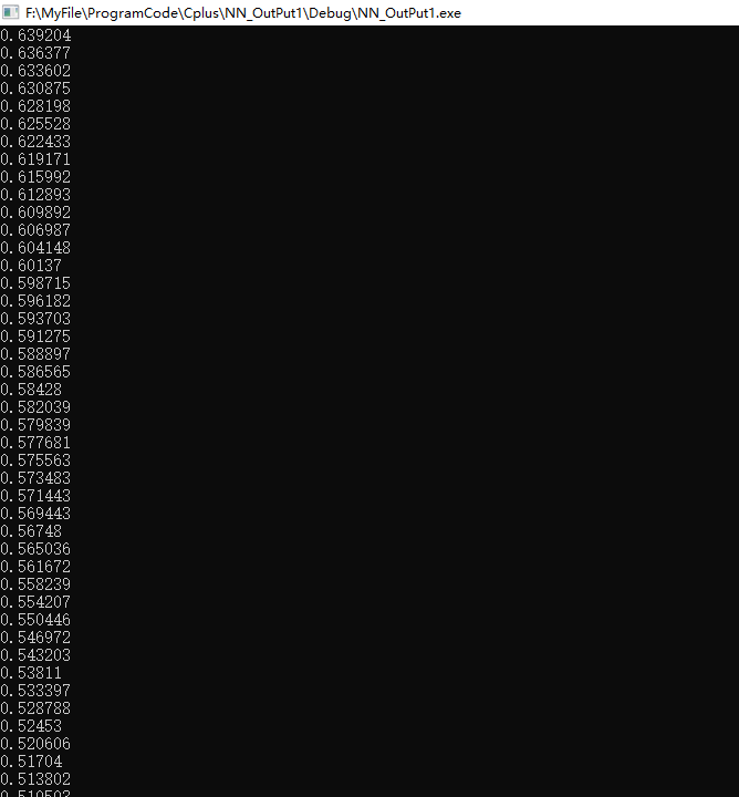
It can be seen that loss is declining steadily.
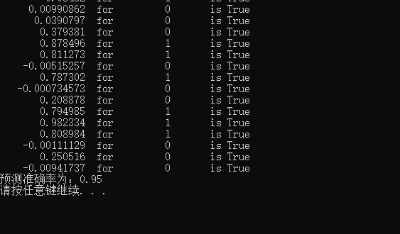
After iteration 2000:
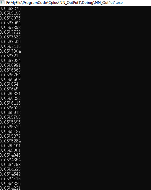
Comparing the predicted results with the real results, it is considered that the correct judgment condition is: y_true is 1, corresponding to y_ PRED > 0.5, otherwise y_true is 0, corresponding to y_ pred<0.5.
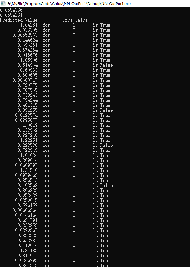
Final accuracy 95%
After several days of writing and several versions, we finally realized the function. It's always easier to know than to do. The code is uploaded here https://github.com/tian0zhi/Neural-Network-By-C-Plus-Plus , use and reprint, please indicate the source