Original link: http://tecdat.cn/?p=17526

This paper proposes an algorithm, which can switch between mean regression and trend following strategy according to market volatility. Two models are studied: one uses historical volatility and the other uses Garch (1,1) volatility prediction. The mean regression strategy uses RSI (2) for modeling: it is Long when RSI (2), otherwise it is Short. The trend tracking strategy is cross modeled with SMA 50/200: when SMA (50) > SMA (200), it is Long, otherwise it is Short.

The following code loads historical prices from Yahoo Finance and compares the effects of buy and hold, mean regression and trend tracking strategies:

    #*****************************************************************
    # Load historical data
    #******************************************************************
    load.packages('quantmod')  
    tickers = 'SPY'
 
    data <- new.env()
    getSymbols(tickers, src = 'yahoo', from = '1970-01-01', env = data, auto.assign = T)
       
    #*****************************************************************
    # Code strategy
    #******************************************************************
    prices = d
    # Buy and hold
    data$weight\[
         
    # Mean regression (MR) strategy
    rsi2 = bt.apply.ma
         
    # Trend tracking (TF) strategy
    sma.short = apply.matrix(prices, SMA, 50)
    sma.long = apply.matrix(prices, SMA, 200)
    data$weight\[\] = NA

    #*****************************************************************
    # Create report
    #******************************************************************
    plotb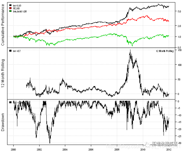

Next, let's create a strategy that switches between mean regression and trend following strategies based on historical market volatility.

#*****************************************************************
＃Regional system transfer according to historical market fluctuations
＃Current volatility is classified as a percentage using a 252 day backtracking period
#******************************************************************

 
# District system transfer history
data$weight\[\] = NA
    data$weight\[\] = iif(vol.rank > 0.5,
                iif(rsi2 <

l=capital, trade.summary=T)
 
#*****************************************************************
#Create report
#******************************************************************
report(regime, mr)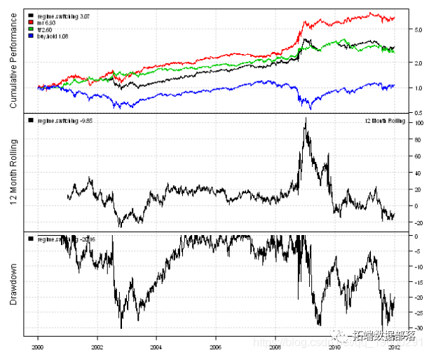

Next, we create a GARCH (1,1) volatility forecast.

There are some R packages that can fit the GARCH model. I will consider the GARCH function in the tseries package and the garchFit function in the fGarch package. The GARCH function in the tseries package is fast, but it can't always find a solution. The garchFit function in the fGarch package is slower, but converges more consistently. To demonstrate the speed difference between the GARCH function and the garchFit function, I created a simple benchmark:

#*****************************************************************
# Garch benchmarking algorithm
#******************************************************************
temp = garchSim(n=252)
 
test1 <- function() {
    fit1=garch(temp, order = c(1, 1), control = garch.control(trace = F))
}
test2 <- function() {
    fit2=garchFit(~ garch(1,1), data = temp, include.mean=FALSE, trace=F)
}
         
benchmark(
    test1(),
    test2(),
    columns=
)

garchFit function is 6 times slower than garch function on average. Therefore, to predict volatility, I will try to use the garch function when finding a solution, otherwise I will try to use the garchFit function.

#*****************************************************************
#Using Garch to predict volatility
#garch from tseries is fast, but it does not always converge
#The garchFit speed of fGarch is slow, but the convergence is consistent
#******************************************************************
load.packages('tseries,fGarch')
         
# Sigma\[t\]^2 = w + a* Sigma\[t-1\]^2 + b*r\[t-1\]^2
garch.predict.one.day <- function(fit, r1) {
    hl = tail( fitted(fit)\[,1\] ,1)    
 
# Same as forecast (fit, n.ahead=1, doplot=F)\[3 \]
garchFit.predict.one.day <- funct
 
garch.vol = NA * hist.vol
for( i in (252+1):nperiods 

 err ) FALSE, warning=function( warn ) FALSE )
                     
    if( !is.logical( fit 

garch(1,1), data = temp, include.mean=FALSE, trace=F),
                    error=function( err ) FALSE, warning=function( warn ) FALSE )
                     
        if( !is.logical(

Now, let's create a strategy that switches between mean regression and trend tracking strategies based on GARCH (1,1) volatility prediction.

#*****************************************************************
# District transfer using Garch
#******************************************************************        
vol.rank = percent.rank(SMA(percent.rank(garch.v
# District transfer Garch
data$weight\[\] = NA
    data$weight\[\] = iif(vol.rank > 0.5,
                iif(rsi2 < 50, 1, -1),
                iif(sma.short > sma.l



#*****************************************************************
#Create report
#******************************************************************
report(regime.switching)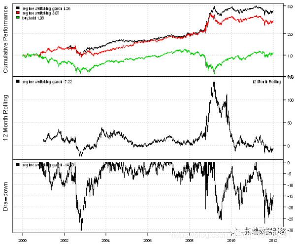

The conversion strategy using GARCH (1,1) volatility prediction is slightly better than that using historical volatility.

You can incorporate forecasts into models and trading strategies in a number of different ways. R has a very rich set of software packages for modeling and predicting time series.

This paper is an excerpt from "R language regional system transfer trading strategy based on Garch Volatility Prediction"