machine learning

Chapter 1: Fundamentals of machine learning Chapter 2: linear regression Chapter 3: logical regression Chapter 4: BP neural network Chapter 5: convolutional neural network Chapter 6: cyclic neural network Chapter 7: decision tree and random forest Chapter 8: support vector machine Chapter 9: Hidden Markov Chapter 10: clustering and other algorithms

Exercises based on Wu Enda's machine learning

Logistic regression github address

preface

Machine learning is an important branch of artificial intelligence and the key to realize intelligence

1, Basic concepts

   logistic regression is also called generalized linear regression model. The biggest difference between it and linear regression model is that their dependent variables are different. If they are continuous, they are multiple linear regression; If it is a binomial distribution, it is logistic regression.
   although the name of Logistic regression is "regression", it is actually a classification method, It is mainly used for two classification problems (that is, there are only two outputs, representing two categories respectively). Logical regression is such a process: facing a regression or classification problem, establish a cost function, and then iteratively solve the optimal model parameters through the optimization method, and then test and verify the quality of our model.
Step:
   (1) find h function (i.e. prediction function);
   (2) construct J function (loss function);
   (3) find a way to minimize the J function and obtain the regression parameters( θ)
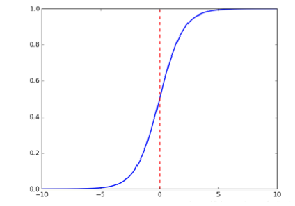
   the graph of the relationship between the probability and the independent variable of the binary classification problem is often an S-shaped curve, which is realized by Sigmoid function in the form of:
         
The constructed prediction function is:
       
   the function output of sigmoid is between (0, 1) and the middle value is 0.5. The meaning of the formula is well understood because the output is between (0, 1) indicates the probability that the data belongs to a certain category. For example, < 0.5 indicates that the current data belongs to class A; > 0.5 indicates that the current data belongs to class B. therefore, we can regard the sigmoid function as the probability density function of the sample data.
   sigmoid function diagram

2, Construct loss function

   and multiple linear regression least square method Corresponding to the parameter estimation method, Maximum likelihood method It is a parameter estimation method used in logistic regression. Its principle is to find such a parameter, which can maximize the possibility that the observed values contained in the sample data can be observed. This method of finding the maximum possibility needs repeated calculation and has high requirements for computing power. The advantages of maximum likelihood method are that the estimation of parameters in large sample data is stable, the deviation is small and the estimation variance is small.
  next, we use probability theory maximum likelihood estimation To solve the loss function.
  first get Probability function Is:
           
Because the sample data (m pieces) are independent, their joint distribution can be expressed as the product of each marginal distribution, and the likelihood function is:

Take the log likelihood function:

Maximum likelihood estimation is required to make L( θ) Maximum value θ， Here, the gradient rise method can be used to solve the problem θ Is the best parameter required:

Based on the maximum likelihood estimation, the cost function and loss function are derived as follows:

3, Solving the minimum value by gradient descent method

(1) θ Update process:
      
      
θ The update process can be written as:
      
(2) Vectorization
   the matrix form of training data is as follows, each line of x has a training sample, and each column has different special values:

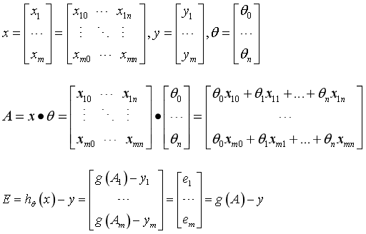
The parameter A of g(A) is A column vector, so when implementing the g function, it is necessary to support the column vector as the parameter and return the column vector. θ The update process can be changed to:

(3) Regularization
Overfitting means overfitting the training data, which increases the complexity of the model and makes the prediction ability of unknown data poor
The left figure shows under fitting, the middle figure shows appropriate fitting, and the right figure shows over fitting.

Regularization is the realization of structural risk minimization strategy, which adds a regularization term or penalty term to the empirical risk. The regularization term is generally a monotonic increasing function of model complexity. The more complex the model is, the larger the regularization term is.
The regular term can take different forms. In the regression problem, take the square loss, which is the L2 norm of the parameter, or take the L1 norm. When taking the square loss, the loss function of the model becomes:

Regularized gradient descent algorithm θ The update for becomes:

4, Regularized logistic regression

# Import data
import pandas as pd
import matplotlib.pyplot as plt
import numpy as np
data=pd.read_csv('ex2data2.txt',header=None,names=['test1','test2','Accepted'])
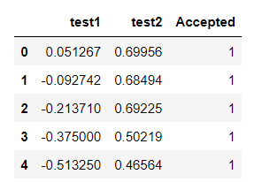
data.head()

Use head() to view data:

# Dataset visualization
positive=data[data['Accepted'].isin([1])]
negative=data[data['Accepted'].isin([0])]
fig,ax=plt.subplots(figsize=(10,10))
ax.scatter(positive['test1'],positive['test2'],label='Accepted = 1',marker='+',s=50,c='black')
ax.scatter(negative['test1'],negative['test2'],label='Accepted = 0',marker='o',s=50,c='y')
ax.legend()
ax.set_xlabel('Microchip Test 1')
ax.set_ylabel('Microchip Test 2')
plt.show()

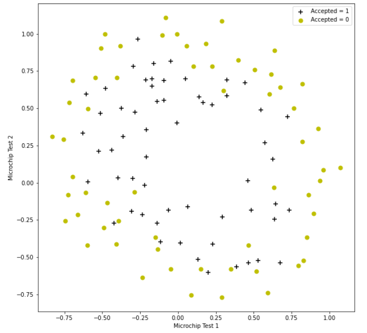
Here we will find that it is difficult to classify this data set, but we can still classify it by logistic regression

One way to better fit data is to create more features from each data point. We will map these features to all polynomial terms of x1 and x2 up to the sixth power.

Next, we use a polynomial of power 6 for mapping:

If the sample size is large, we have to use logistic regression to solve the problem, which is undoubtedly very complex. In our example, the original features are X1 and X2, which can create more features x1,x2, x1x2, x12, x22,... X1nX2n with polynomials. Because more features are used for logistic regression, the obtained segmentation line can be the shape of any higher-order function. (but this will also lead to the problem of over fitting, which we will talk about later) feature mapping. If you understand the principle of feature mapping, you will have the answer. If the feature is mapped to the 6th power, you can get 1 + 2 + 3 + 4 + 5 + 6 + 7 = 28 features. If you don't understand, see the following:

1

x1, x2

x12 , x1x2, x22

x12x2, x1x22, x13, x23

x13x2, x12x22, x1x23, x14 , x24

x14x2, x13x22, x12x23, x1x24 , x15 , x25

x15x2, x14x22, x13x23 , x12x24 , x1x25 , x16 , x26

# feature mapping
def feature_mapping(x1, x2, power):
    data = {}   
    for i in np.arange(power + 1):    #When i=n, it is all combinations of n-powers. Up to power in total
        for p in np.arange(i + 1):
            data["f{}{}".format(i - p, p)] = np.power(x1, i - p) * np.power(x2, p) 
    return pd.DataFrame(data) 
x1 = data['test1'].values   #Define the data of x1 and x2
x2 = data['test2'].values
data2 = feature_mapping(x1, x2, power=6)
data2.head()

data2.describe()

#Convert 2D table to array format
X = data2  
y = data['Accepted']
theta = np.zeros(X.shape[1])
X.shape,y.shape,theta.shape

The ideal results can be obtained here: ((118, 28), (118,), (28,))

#Define regularization cost function
def costReg(theta, X, y,l=1):    
    first = (-y) * np.log(sigmoid(X @ theta)) 
    second = (1 - y)*np.log(1 - sigmoid(X @ theta))
    cost=np.mean(first - second)
    reg=(l / (2 * len(X))) *(theta[1:] @ theta[1:])  
    return cost+reg

#Define activation function
def sigmoid(z):  
    return 1 / (1 + np.exp(- z))

costReg(theta, X, y,l=1)

The ideal condition here is 0.6931471805599461

#Define the gradient update of regularization
def gradientReg(theta, X, y ,l=1):   
    grad=(X.T @ (sigmoid(X @ theta) - y))/len(X)
    reg = (1 / len(X)) * theta
    reg[0]=0
    #Similarly, the first one will not be punished θ
    return grad + reg
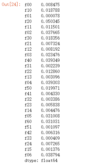
gradientReg(theta, X, y ,l=1)

Here you can get:

#Then we perform gradient descent through advanced optimization
import scipy.optimize as opt
# result=opt.fmin_tnc(func=costReg,x0=theta,fprime=gradientReg,args=(X,y,2))
res = opt.minimize(fun=costReg, x0=theta, args=(X, y), method='Newton-CG', jac=gradientReg)
res
res.x

Here we use res.x to see our final theta:
array([ 1.27274175, 0.62527239, 1.18108994, -2.01996653, -0.91742318,
-1.43166726, 0.12400716, -0.36553523, -0.35723936, -0.17513155,
-1.45815693, -0.05098901, -0.61555554, -0.27470685, -1.19281737,
-0.24218799, -0.2060068 , -0.04473071, -0.27778419, -0.2953783 ,
-0.45635874, -1.04320168, 0.02777154, -0.29243171, 0.01556673,
-0.32737987, -0.14388645, -0.92465133])

#We use the updated theta to calculate the classification accuracy
final_theta = res.x
def predict(theta, X):
    probability = sigmoid(X@theta)
    return [1 if x >= 0.5 else 0 for x in probability] 
predictions = predict(final_theta, X)
correct = [1 if a==b else 0 for (a, b) in zip(predictions, y)]  
accuracy = sum(correct) / len(correct)
accuracy

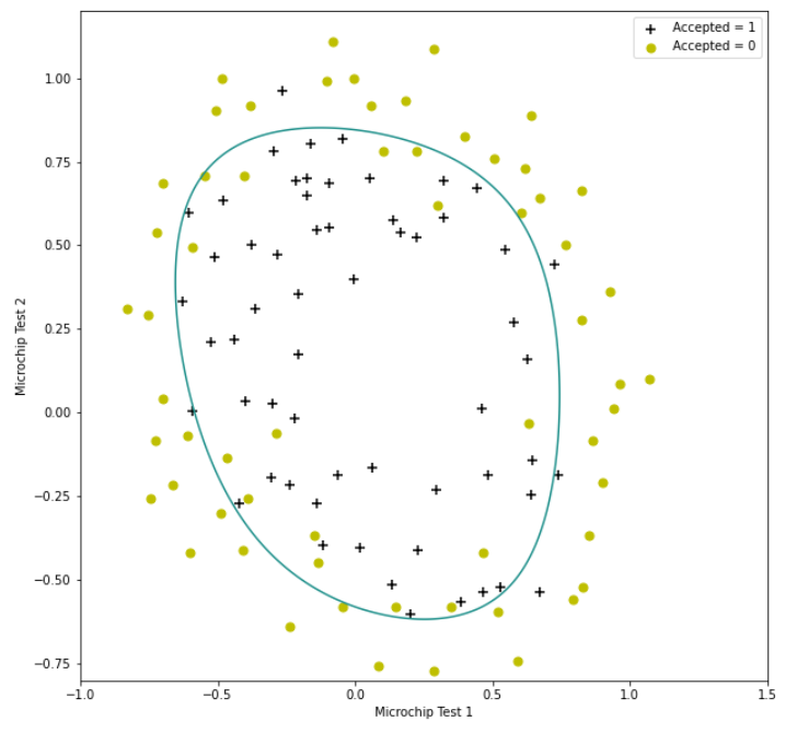
Ideally, 0.83050845762712 is obtained

positive=data[data['Accepted'].isin([1])]
negative=data[data['Accepted'].isin([0])]
fig,ax=plt.subplots(figsize=(10,10))
ax.scatter(positive['test1'],positive['test2'],label='Accepted = 1',marker='+',s=50,c='black')
ax.scatter(negative['test1'],negative['test2'],label='Accepted = 0',marker='o',s=50,c='y')
ax.legend()
ax.set_xlabel('Microchip Test 1')
ax.set_ylabel('Microchip Test 2')
x = np.linspace(-1, 1.5, 250)  
xx, yy = np.meshgrid(x, x)  
z = feature_mapping(xx.ravel(), yy.ravel(), 6).values 
z = z @ final_theta  
z = z.reshape(xx.shape)  
plt.contour(xx, yy, z, 0) 
plt.ylim(-.8, 1.2)
plt.show()  

summary

This is equivalent to my practice of Wu Enda's regularized logical regression, which should be very clear. I look forward to discussing it with you.