1. Project source

(1) Thesis title

The reproduced paper: Joint Face Detection and Alignment using Multi-task Cascaded Convolutional Networks , the original author implemented the algorithm using Matlab.

(2) Achieve goals

The task of this time is based on the pytoch implementation of this paper, which is reproduced using Baidu paste paste framework. This blog is based on the Pytorch reproduction of the paper to learn and analyze MTCNN papers and algorithms.

(3) Related resources

Download the following resources as required:

• Refer to Github's reproduction code and make a little modification yourself
  Baidu online disk: https://pan.baidu.com/s/14otWIZM8ix-dNoBkCYGoiA
  Extraction code: xwet

• WIDER FACE Wider in dataset_ face_ split. Zip and leader_ train. Zip compressed package. The storage paths after decompression are:
  MTCNN_TUTORIAL-MASTER/data_set/wider_face_split/
  MTCNN_TUTORIAL-MASTER/data_set/WIDER_train/

• Sign in FDDB official website Download data sets, including Original images and Face annotations, which are stored in the following paths:
  MTCNN_TUTORIAL-MASTER/data_set/train/
  MTCNN_TUTORIAL-MASTER/data_set/FDDB-folds/

2. Code operation

Since the training and testing process of each stage in this paper is cascaded according to the sequence of PNET rnet onet, and the training results of the previous stage are the network input of the later stage, the training and testing need to be carried out in multiple stages. The following will briefly analyze each stage one by one.

i) Image annotation

On mtcnn_ TUTORIAL-MASTER/data_ Create a new folder anno under preprocessing / folder_ Store and execute the following instructions

python data_preprocessing/transform.py

The file anno will be generated under this path_ train. txt to download the pre downloaded wider_ face_ split/wider_ face_ train. The mat tag file is converted to txt format.
Converted wider_face_train.txt file records the original image address in the dataset and the face frame coordinates as the ground truth.

ii) generate PNet training data

Input the training data of PNet and divide it into three parts according to the value of image intersection and union ratio IOU: 0-0.3 is divided into negative, 0.4-0.65 is divided into part and 0.65-1 is divided into positive.
Execute the following instructions

python data_preprocessing/gen_Pnet_train_data.py

The file is responsible for crop out the image from the original image, classify it according to the IOU value, and store the data of the three labels into data respectively_ set/train/12/negative/，data_set/train/12/part/，data_set/train/12/positive/
--------------------------------------A split line-------------------------------------------
Then execute the following instructions

python data_preprocessing/assemble_Pnet_imglist.py

Assemble the PNet dataset annotation file, complete shuffle and disrupt it, and then complete the preparation of PNet training data

iii) training PNet

Execute the following statement

python train/Train_Pnet.py

In the training process, the train mode and val mode of PNet network are carried out alternately.
It is worth mentioning that before the first training, you need to create the folder data corresponding to the verification set_ Set / Val / 12 /, POS will be generated in the folder_ 12_ val.txt，part_12_val.txt，neg_12_val.txt three annotation files.

iv) generate RNet training data

Create data_set/train/24 / folder, execute the following command

python data_preprocessing/gen_Rnet_train_data.py
python data_preprocessing/assemble_Rnet_imglist.py

The function is roughly the same as that of PNet data preparation in step 2, data_ POS will be generated in the set / train / 24 / folder_ 24_ val.txt，part_24_val.txt，neg_24_val.txt three annotation files

v) Training RNet

Execute the following statements, and the function is roughly the same as the PNet network training in step 3

python train/Train_Pnet.py

vi) generate ONet training data

Create data_set/train/48 / folder, execute the following statements

python data_preprocessing/gen_Onet_train_data.py

The function is the same as the PNet data preparation function in step 2. POS will be generated in the folder_ 48.txt, part_ 48.txt, neg_ 48.txt three annotation files

Since the third stage ONet, i.e. Output Net, needs to output facial landmark coordinates, additional data needs to be generated in the data preparation stage_ preprocessing/anno_ store/landmark_ 48.txt file, record the facial marker point information, and execute the following statements

python data_preprocessing/gen_landmark_48.py

To complete the preprocessing and shuffling of ONet training data, execute the following statements

python data_preprocessing/assemble_Onet_imglist.py

vii) training ONet

Execute the following statements, and the function is roughly the same as the PNet network training in step 3

python train/Train_Onet.py

Since then, the training and verification phase has been completed

Let's show our training process and test results~

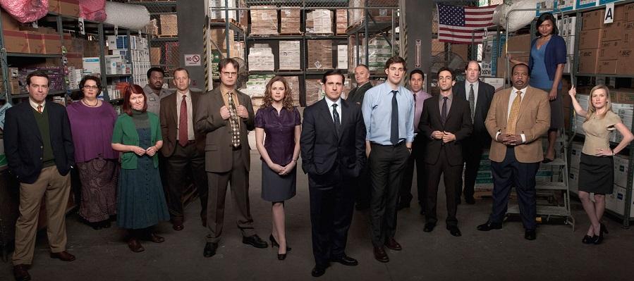
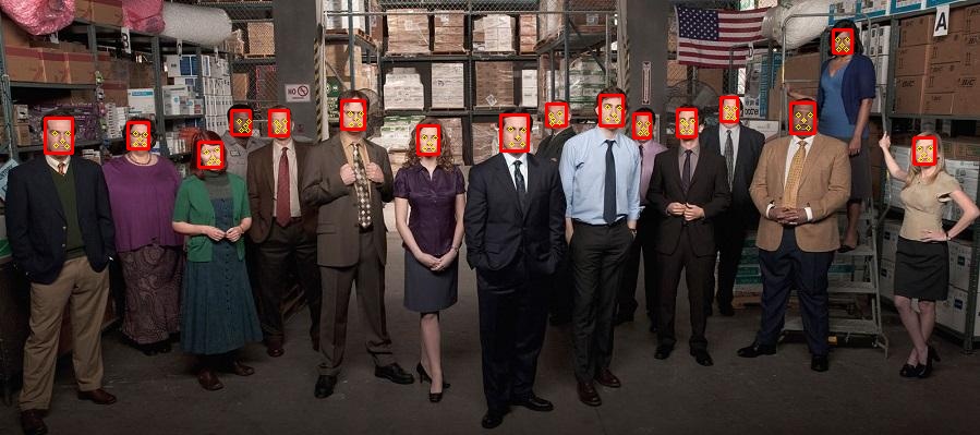
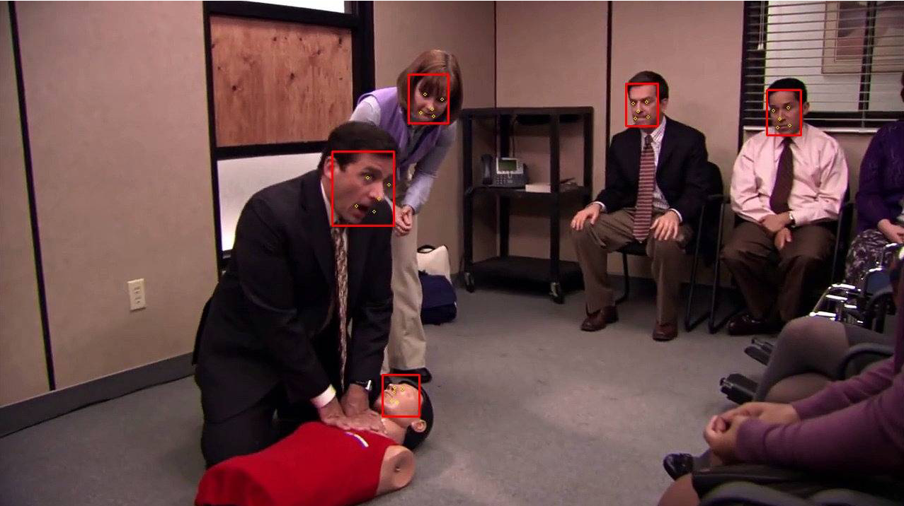
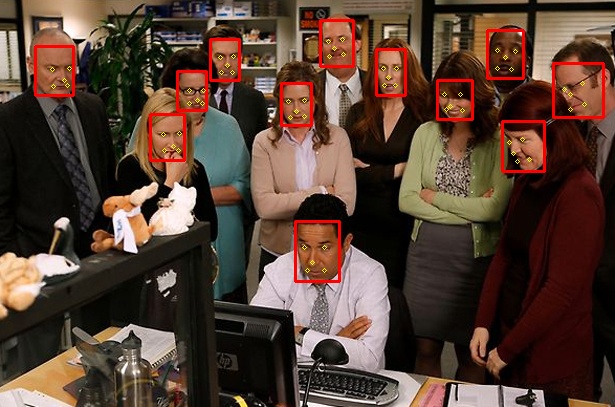
After loading the trained model, we trained for several rounds, and the effect is very good, isn't it~

3. Algorithm and code analysis

Read the paper through the code and make a series of analysis on the model and algorithm.

• On the whole, the whole training process is actually carried out by the three networks iteratively in the order of P-R-O, including training and verification. At the same time, the network as a whole maintains the sequence of data preparation (randomly crop out the image frame for training, and divide it into positive, part and negative according to its IOU value), data disturbance and network training, and the three PRO networks are connected end to end.

• In the training process of the network, each stage calculates the loss value for three tasks: face binary classification, bounding box regression and face key points. As for the selection of loss function, the cross entropy loss function is used for face classification, and the mean square error MSE is used for other problems.
  It is worth mentioning that because the feature map size in PNet and RNet is small, it is difficult to recognize landmarks. Therefore, we only introduce the task of face key point detection in the last ONet, so we only calculate the mean square error of face marker landmarks in the training process of ONet.
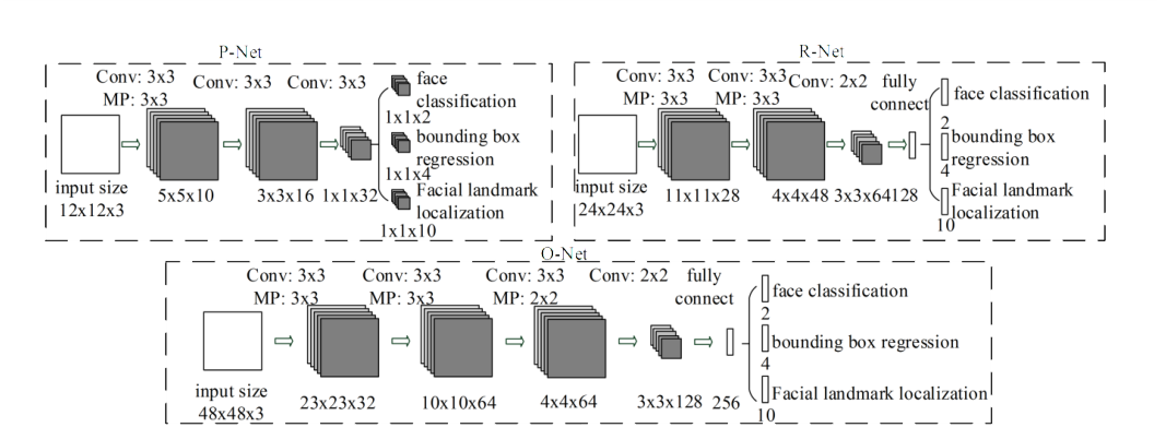
  The following figure may be misleading, which makes you think that the training of landmark task is also carried out in PNet and RNet, but in fact, the author has given a clear answer in the code.
  

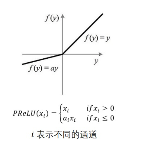
• Based on the above figure, we explain the network architecture: in order to improve the performance of the network, the author uses 3x3 filter instead of 5x5 convolution kernel, and PReLu is used in the activation function, which is about the shape of the following figure.
  As for the specific shape of PRO network, the input data are 12x12x3, 24x24x3 and 48x48x3 respectively. After a series of convolution, pooling, convolution and pooling, the training of backbone network is completed. The training results of Zhigan network are input into two (ONet is three) branches respectively, and different convolution checks are used for training, corresponding to three tasks: face classification, bounding box expression and facial landmark localization.
  It is worth mentioning that in ONet, because it is more complex than P and R networks, an additional convolution layer is set, hoping to gain better performance through the increase of network depth.
  

• In the data preparation stage, the technique of randomly crowding out the sample box, that is, the method of obtaining neg, part and pos samples. In data_preprocessing/gen_Pnet_train_data.py as an example, the code is directly divided into two for loops, one large and one small.
  The following is a small for loop, which is only responsible for taking 35 negative samples (in fact, some negative samples are also obtained in the second for loop)

neg_num = 0
while neg_num < 35:
    # Some square frames of different sizes are randomly crop ped (the minimum side length is 12), and the larger negative is allowed in 35 negative samples
    # Width and height are the width and height of the image
    size = np.random.randint(12, min(width, height) / 2)
    nx = np.random.randint(0, width - size)
    ny = np.random.randint(0, height - size)
    crop_box = np.array([nx, ny, nx + size, ny + size])

    Iou =IoU(crop_box, boxes)

    cropped_im = img[ny: ny + size, nx: nx + size, :]
    #Zoom to a fixed size to facilitate the first stage PNet operation
    resized_im = cv2.resize(cropped_im, (12, 12), interpolation=cv2.INTER_LINEAR)

    if np.max(Iou) < 0.3:
        # Iou with all gts must below 0.3
        save_file = os.path.join(neg_save_dir, "%s.jpg" % n_idx)
        f2.write(save_file + ' 0\n')
        cv2.imwrite(save_file, resized_im)
        n_idx += 1
        neg_num += 1#Find 35 negative samples for each picture

The purpose of this part of the code is to perform random crop in a large range and obtain 35 negative samples. The sample box is a square with a side length greater than 12, and the value range of the box is distributed on the whole picture.

The following is a large for loop. positive, part and negative samples are involved

    # Within the coordinates of ground true
    for box in boxes:
        # box (x_left, y_top, w, h)
        x1, y1, x2, y2 = box
        w = x2 - x1 + 1
        h = y2 - y1 + 1

        # ignore small faces
        # in case the ground truth boxes of small faces are not accurate
        if max(w, h) < 40 or x1 < 0 or y1 < 0 or w < 0 or h < 0:
            continue

        # generate negative examples that have overlap with gt, generate negative samples that coincide with ground true
        for i in range(5):
            size = np.random.randint(12, min(width, height) / 2)
            # delta_x and delta_y are offsets of (x1, y1)

            delta_x = np.random.randint(max(-size, -x1), w)
            delta_y = np.random.randint(max(-size, -y1), h)
            nx1 = max(0, x1 + delta_x)
            ny1 = max(0, y1 + delta_y)

            if nx1 + size > width or ny1 + size > height:
                continue
            crop_box = np.array([nx1, ny1, nx1 + size, ny1 + size])
            Iou = IoU(crop_box, boxes)

            cropped_im = img[ny1: ny1 + size, nx1: nx1 + size, :]
            # Zoom to fixed size
            resized_im = cv2.resize(cropped_im, (12, 12), interpolation=cv2.INTER_LINEAR)

            if np.max(Iou) < 0.3:
                # Iou with all gts must below 0.3
                save_file = os.path.join(neg_save_dir, "%s.jpg" % n_idx)
                f2.write(save_file + ' 0\n')
                cv2.imwrite(save_file, resized_im)
                n_idx += 1

        # generate positive examples and part faces based on ground truth
        for i in range(20):
            size = np.random.randint(int(min(w, h) * 0.8), np.ceil(1.25 * max(w, h)))

            # delta here is the offset of box center
            delta_x = np.random.randint(-w * 0.2, w * 0.2)
            delta_y = np.random.randint(-h * 0.2, h * 0.2)

            nx1 = max(x1 + w / 2 + delta_x - size / 2, 0)
            ny1 = max(y1 + h / 2 + delta_y - size / 2, 0)
            nx2 = nx1 + size
            ny2 = ny1 + size

            if nx2 > width or ny2 > height:
                continue    #Random failure, skip
            crop_box = np.array([nx1, ny1, nx2, ny2])

            # normalization
            offset_x1 = (x1 - nx1) / float(size)
            offset_y1 = (y1 - ny1) / float(size)
            offset_x2 = (x2 - nx2) / float(size)
            offset_y2 = (y2 - ny2) / float(size)

            cropped_im = img[int(ny1): int(ny2), int(nx1): int(nx2), :]
            resized_im = cv2.resize(cropped_im, (12, 12), interpolation=cv2.INTER_LINEAR)

            box_ = box.reshape(1, -1)
            if IoU(crop_box, box_) >= 0.65:#Positive sample
                save_file = os.path.join(pos_save_dir, "%s.jpg" % p_idx)
                f1.write(save_file + ' 1 %.2f %.2f %.2f %.2f\n' % (offset_x1, offset_y1, offset_x2, offset_y2))
                cv2.imwrite(save_file, resized_im)
                p_idx += 1
            elif IoU(crop_box, box_) >= 0.4 and d_idx < 1.2*p_idx + 1:#For part samples, it is expected that the number of part images is more than 1.2 times that of positive samples
                save_file = os.path.join(part_save_dir, "%s.jpg" % d_idx)
                f3.write(save_file + ' -1 %.2f %.2f %.2f %.2f\n' % (offset_x1, offset_y1, offset_x2, offset_y2))
                cv2.imwrite(save_file, resized_im)
                d_idx += 1

The code is very long. It is not explained line by line. On the whole, there is a for loop with two for. For the small for loop, the first for is to try to obtain some negative samples in five iterations, and the second for loop is to strive to obtain some part and positive samples in 20 iterations.
In fact, the large for loop of the whole can be found to be the traversal of the box, that is, the traversal of each ground truth. What is the purpose? Combined with the crop process of three samples, it can be found that this crop takes random values around the correct face frame. In fact, this is a kind of pseudo-random.

An important but easily overlooked point is that the width w and height h in the code are different from the full image size represented by the previous width and height. w and H are the size of the ground truth face frame. In fact, such a value can ensure that the three samples from the cross are located around the correct answer.

As for the significance of this pseudo-random operation, for part and positive samples, the efficiency of obtaining a specified number of samples by taking random values around the correct answer is naturally greater than that in the random frame method of the whole graph; For the negative samples, the negative samples obtained by crop around the correct answers may be more confusing. It is a natural "difficult sample", which coincides with the concept of "difficult sample mining" in the follow-up code.

The reason why the number of cycles is 5 and 20 respectively is that the proportion of various samples roughly meets the requirements of negatives: positions: part (: landmark) = 3:1:1 (: 2)

• In fact, there is another question: why does the face frame have to choose a square? After all, there should still be a few meat faces that are fat and round. Maybe you can try to keep the width unchanged in the process of subsequent code improvement, and multiply the length by a coefficient greater than 1. If the aspect ratio of the face is about 1.5:1, it may be more reasonable. After all, the selection of the shape of the face frame will also affect the calculation of IOU, and the square frame will inevitably lead to a smaller calculation value of IOU, Maybe this will affect the sensitivity of the model. We will try to improve this factor in the later model reproduction.
  In fact, I haven't seen a lot of images in the dataset, hahaha, but I guess the author may have this idea, but the faces in the dataset often have different tilt angles. In this case, the inclusiveness of squares is obviously greater than that of rectangles. If so, the author should be on the fifth floor ~ ~ as for the specific choice, Different data sets should have different biases, or should they be proved by summarizing the characteristics of data sets and experiments. In general, we will try to improve this factor in the later model reproduction!
• As for the implementation of difficult sample mining, the author rewrites the loss function through ohem thought. In the process of loss function operation, the first 70% samples with loss value are only applied in the process of back propagation and gradient descent, which is what we call difficult samples. It's very smart, isn't it~
• I found that the nms mentioned in the paper, i.e. non maximum suppression, was only seen in the network example test code, but its application was not seen in the training process. I haven't figured this out yet. I may discuss it with my teammates and teachers.