1. Structure
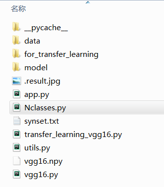
The image above is a replication of all the files of vgg16. The data folder is a test image. This replication only calls another trained model to identify the picture.vgg16.py reproduces the network structure of vgg16 and imports trained model parameters.Utils.pyFor input picture preprocessing program,Nclasses.py Is the label given to each image and the corresponding index value.App.pyIs our call file for image recognition.
2. Code Details
1,vgg16.py
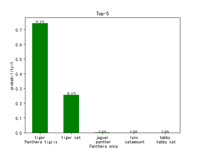
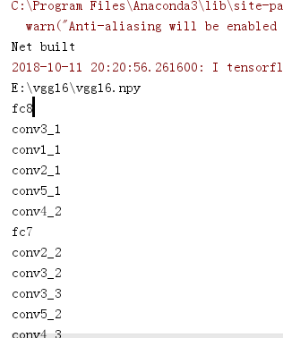
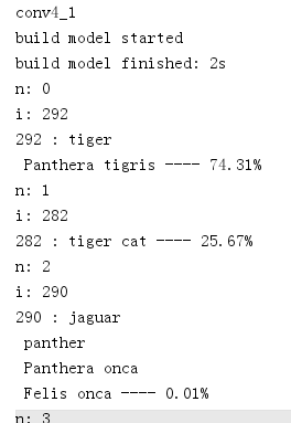
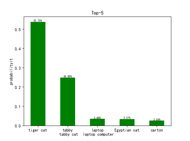
  1 import tensorflow as tf
  2 import numpy as np
  3 import os
  4 import time
  5 import matplotlib.pyplot as plt
  6 from Nclasses import labels
  7
  8 VGG_MEAN = [103.939,116.779,123.68] #sample RGB Average
  9
 10 class Vgg16:
 11     def __init__(self,vgg16_npy_path=None):
 12         if vgg16_npy_path is None:
 13             vgg16_npy_path = os.path.join(os.getcwd(),'vgg16.npy') # os.getcwd() Method is used to return the current working directory.
 14             print(vgg16_npy_path)
 15         # Traversing key-value pairs,Import Model Parameters
 16         self.data_dict = np.load(vgg16_npy_path,encoding='latin1').item() # Load here vgg16.npy Parameters
 17         # ergodic data_dict Each key in
 18         for i in self.data_dict:
 19             print(i)
 20     #Forward Propagation Model
 21     def inference(self,images):
 22         start_time = time.time() # Get the start time of forward propagation
 23         print('build model started')
 24         ## Multiply 255.0 pixels by pixels (according to the initialization steps described in the original paper)
 25         images_scaled = images * 255
 26         # from GRB Convert color channels to BGR,Also available cv In GRBtoBGR
 27         #tf.split()Put the rgb Channel Separation
 28         red,green,blue = tf.split(images_scaled,num_or_size_splits=3,axis=3)
 29         # Subtracts the average pixel value for each channel by sample, which removes the average brightness value of the image. This method is commonly used on gray-scale images.
 30         bgr = tf.concat(values=[
 31             blue-VGG_MEAN[0],
 32             green-VGG_MEAN[1],
 33             red-VGG_MEAN[2]
 34         ],axis=3)
 35
 36
 37         #structure vgg network structure
 38         ## Next, build a 16-layer network of VGG Gs (with 5 convolutions and 3 full connections) and read network parameters layer by layer from the namespace
 39         # The first convolution, consisting of two convolution layers followed by a maximum pooling layer, is used to reduce the size of the picture
 40         # Incoming namespace name,To get the convolution kernel and offset of the layer, do the convolution, and return the value after the activation function
 41         conv1_1 = self.conv_layer(bgr,'conv1_1')
 42         conv1_2 = self.conv_layer(conv1_1,'conv1_2')
 43         # According to the incoming pooling Name pooling the layer accordingly
 44         pool1 = self.max_pool(conv1_2,'pool1')
 45
 46         #Second layer convolution
 47         # The following forward propagation process is the same as the first one
 48         # The second convolution contains two convolution layers, one maximum pooled layer
 49         conv2_1 = self.conv_layer(pool1,'conv2_1')
 50         conv2_2 = self.conv_layer(conv2_1,'conv2_2')
 51         pool2 = self.max_pool(conv2_2,'pool2')
 52         # The third convolution, consisting of three convolution layers and one maximum pooled layer
 53         conv3_1 = self.conv_layer(pool2,'conv3_1')
 54         conv3_2 = self.conv_layer(conv3_1,'conv3_2')
 55         conv3_3 = self.conv_layer(conv3_2,'conv3_3')
 56         pool3 = self.max_pool(conv3_3,'pool3')
 57         # The fourth convolution, which consists of three convolution layers and one maximum pooled layer
 58         conv4_1 = self.conv_layer(pool3,'conv4_1')
 59         conv4_2 = self.conv_layer(conv4_1,'conv4_2')
 60         conv4_3 = self.conv_layer(conv4_2,'conv4_3')
 61         pool4 = self.max_pool(conv4_3,'pool4')
 62         # Segment 5 convolution, consisting of three convolution layers and one maximum pooled layer
 63         conv5_1 = self.conv_layer(pool4, 'conv5_1')
 64         conv5_2 = self.conv_layer(conv5_1, 'conv5_2')
 65         conv5_3 = self.conv_layer(conv5_2, 'conv5_3')
 66         pool5 = self.max_pool(conv5_3, 'pool5')
 67         # Layer 6 Full Connection
 68         #Full Connection Layer
 69         fc6 = self.fc_layer(pool5,'fc6') # According to Namespace name Do weighted sum operation
 70         fc6_relu = tf.nn.relu(fc6)
 71         fc7 = self.fc_layer(fc6_relu,'fc7')
 72         fc7_relu = tf.nn.relu(fc7)
 73         fc8 = self.fc_layer(fc7_relu,'fc8')
 74         # After the last layer is fully connected, do it again softmax Classify and get the probability of belonging to each category
 75         self.out = tf.nn.softmax(fc8,name='prediction')
 76
 77         # Empty the dictionary of model parameters obtained this time to end the forward propagation time
 78         self.data_dict = None
 79         print(("build model finished: %ds" % (time.time() - start_time)))
 80
 81     #Create convolution layer function, convolution kernel, offset from vgg16.npy Get in
 82     def conv_layer(self,conv_in,name):
 83         with tf.variable_scope(name): # Finding network parameters for the corresponding convolution layer from the namespace
 84             conv_W = tf.constant(self.data_dict[name][0],name= name + '_filter') # Read the convolution core of this layer
 85             conv_biase = tf.constant(self.data_dict[name][1],name= name + '_biases') # Read offset
 86             conv = tf.nn.conv2d(conv_in,conv_W,strides=[1,1,1,1],padding='SAME') # Convolution calculation
 87             return tf.nn.relu(tf.nn.bias_add(conv,conv_biase)) # Add offset and do activation calculation
 88
 89     #Maximum pooled layer
 90     def max_pool(self,input_data,name):
 91         return tf.nn.max_pool(input_data,ksize=[1,2,2,1],strides=[1,2,2,1],padding='SAME',name=name)
 92
 93     #Average pooled layer
 94     def avg_pool(self, input_data, name):
 95         return tf.nn.avg_pool(input_data, ksize=[1, 2, 2, 1], strides=[1, 2, 2, 1], padding='SAME', name=name)
 96
 97     # Define forward propagation calculation for fully connected layers
 98     def fc_layer(self,input_data,name):
 99         fc_W = tf.constant(self.data_dict[name][0],name=name + '_Weight')
100         fc_b = tf.constant(self.data_dict[name][1],name=name + '_b')
101
102         shape = input_data.get_shape().as_list() #Get a list of input dimension information
103         dim =1
104         for i in shape[1:]:
105             dim *= i # Multiply the dimensions of each layer, that is, long*wide*Number of Channels
106         # Changing the shape of the signature graph, that is, stretching the resulting multidimensional signatures only into the sixth fully connected layer
107         input_data = tf.reshape(input_data,[-1,dim])
108
109         return tf.nn.bias_add(tf.matmul(input_data,fc_W),fc_b) # Weighted sum with offset for this layer of input
110
111     # Define percentage conversion function
112     def percent(self,value):
113         return '%.2f%%' % (value * 100)
114     #Judging Picture Category Function
115     def test(self,file_path,prob):
116         #Define a figure Draw the window and specify the name of the window. You can also set the size of the window
117         fig = plt.figure(u"Top-5 Forecast results")
118         synset = [l.strip() for l in open(file_path).readlines()]
119
120         # argsort Function returns index values from smallest to largest array values
121         # np.argsort The function returns the predicted value ( probability Data structure[[Probability values for each prediction category]])Index values from small to large,
122         # Five index values with the highest probability of prediction are extracted.
123         top5 = np.argsort(prob)[-1:-6:-1]
124         #print(pred)
125
126         # Define two list---Corresponding probability values and actual labels ( zebra)
127         values = []
128         bar_label = []
129         # Five possibilities for large output probability groups,And list them one by one with the label
130         for n, i in enumerate(top5):
131             print("n:", n)
132             print("i:", i)
133             values.append(prob[i])# Remove and place the predicted probability value corresponding to the index value values
134             bar_label.append(labels[i]) # Remove the actual label according to the index value and put it in bar_label
135             # Probability of belonging to this category
136             print(i, ":", labels[i], "----", self.percent(prob[i])) # Print probability of belonging to a category
137         # Column Chart Processing
138         ax = fig.add_subplot(111) # Divide the canvas into rows and columns and place the following image in them
139         # bar()Function plots a column graph with parameters range(len(values)Is the column subscript, values A list of column heights (that is, five predicted probability values,
140         # tick_label Is the label displayed on each column (the actual label), width Is the width of the column, fc Is the color of the column)
141         ax.bar(range(len(values)), values, tick_label=bar_label, width=0.5, fc='g')
142         ax.set_ylabel(u'probabilityit') # Set Horizontal Axis Label
143         ax.set_title(u'Top-5') # Add Title
144         for a, b in zip(range(len(values)), values):
145             # Add a corresponding prediction probability value at the top of each column. a, b Represents coordinates, b+0.0005 Indicates that text information is to be placed above the top of each column
146             # 0.0005 Location,
147             #  center Is the middle position indicating that the text is located horizontally at the top of the column. bottom Place text horizontally at the bottom of the vertical direction of the top of the column
148             # Location, fontsize Is Font Size
149             ax.text(a, b + 0.0005, self.percent(b), ha='center', va='bottom', fontsize=7)
150         plt.savefig('.result.jpg')  # Save Pictures
151         plt.show()# Pop-up window display image
In this section, we have created the forward propagation of VGG16 network structure, including convolution core, offset, pooling layer and full connection layer. What we need to mention here is the establishment of full connection layer. To create a full connection layer, we first need to read the dimension information list of that layer, then we need to change the shape of the feature map and stretch the multidimensional features that will be obtained in the sixth layer.Make it conform to the input of the fully connected layer, where the shape has elements [-1], flattening the dimension to one dimension for the purpose of dimension reduction.
2,utils.py
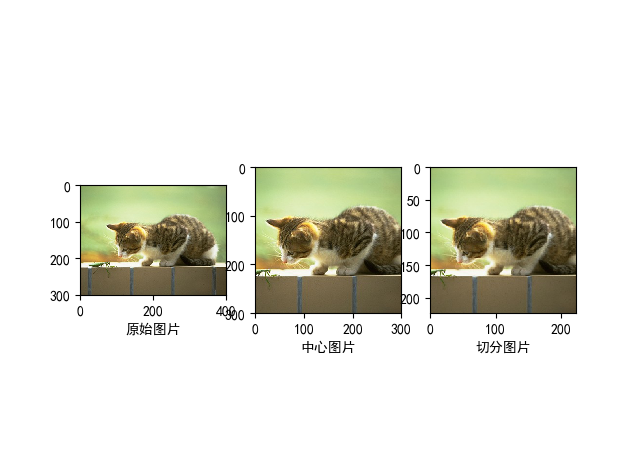
from skimage import io, transform
import numpy as np
import matplotlib.pyplot as plt
import tensorflow as tf
from pylab import mpl
import os
mpl.rcParams['font.sans-serif']=['SimHei'] # Normal display of Chinese labels
mpl.rcParams['axes.unicode_minus']=False # Display plus and minus sign normally

def load_image(path):
    fig = plt.figure('Center and Resize')

    img = io.imread(path) # Read pictures from incoming paths
    img = img / 255.0 # Normalize pixels to[0,1]
    ax0 = fig.add_subplot(131)
    ax0.set_xlabel(u'Original Picture')  # Add Sublabel
    ax0.imshow(img)
    ## Image processing section
    #Subtract the width and height of the picture from the shortest edge and average it to take out the center image
    short_edge = min(img.shape[:2]) # Find the shortest edge of the image
    y = int((img.shape[0] - short_edge) // 2)
    x = int((img.shape[1] - short_edge)// 2)
    crop_img = img[y:y + short_edge,x:x + short_edge] #Remove the sliced central image

    ax1 = fig.add_subplot(132)
    ax1.set_xlabel(u"Center Picture")
    ax1.imshow(crop_img)

    #Central image resize 224, 224
    resized_img = transform.resize(crop_img,(224,224))

    ax2 = fig.add_subplot(133)
    ax2.set_xlabel('Divide pictures') # Add Sublabel
    ax2.imshow(resized_img)

    #plt.show()

    img_read = resized_img.reshape((1,224,224,3))  # shape [1, 224, 224, 3]
    return img_read

def load_data():
    imgs = {'tiger':[],'kittycat':[]}
    for k in imgs.keys():
        dir = './data/' + k
        for file in os.listdir(dir):
            if not file.lower().endswith('.jpg'):
                continue
            try:
                resized_img = load_image(os.path.join(dir,file))
            except OSError:
                continue

            imgs[k].append(resized_img)    # [1, height, width, depth] * n
            if len(imgs[k]) == 2:          # only use 400 imgs to reduce my memory load
                break

    return imgs['tiger'],imgs['kittycat']
In this part, the input pictures are processed, clipped, scaled, etc. to meet the needs of network input. The main idea is to normalize the image and process it, the results are as follows:
3,app.py
 1 import numpy as np
 2 import tensorflow as tf
 3 import matplotlib.pyplot as plt
 4 import vgg16
 5 import utils
 6 #Input of image to be detected and preprocessed
 7 batch = utils.load_image(r'E:\vgg16\for_transfer_learning\data\kittycat/000129037.jpg')
 8
 9 #Define a figure Draw the window and specify the name of the window. You can also set the size of the window
10 fig = plt.figure(u"Top-5 Forecast results")
11 print('Net built')
12 with tf.Session() as sess:
13     # Define a dimension as[?,224,224,3],Type is float32 Of tensor placeholder
14     images = tf.placeholder(tf.float32, [None, 224, 224, 3])
15     feed_dict = {images: batch}
16     #class Vgg16 Instantiate vgg
17     vgg = vgg16.Vgg16()
18     # Call member methods of classes inference(),And pass in the image to be tested, which is also the process of network forward propagation
19     vgg.inference(images)
20     ## Feed a batch's data into the network to get the predicted output of the network
21     probability = sess.run(vgg.out, feed_dict=feed_dict)
22
23     vgg.test('./synset.txt',probability[0])
This part calls the above programs to identify the image. What we need to do is call the network structure of VGG16, then calculate the probability, the five possibilities of the highest output probability, and one-to-one correspondence with the label, and finally draw the result with a column chart to express the result.
3. Testing
FunctionApp.pyReplace the picture directory in batch with the one you want to recognize
first group
Group 2