concept

Computer architecture

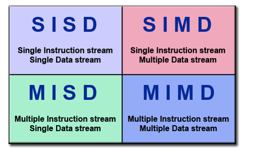
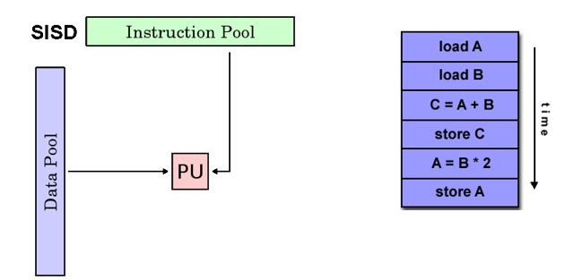
SISD

• Single instruction stream Single Data stream
• Single instruction single data, serial computer
• In any clock cycle, the CPU has only one instruction stream; In any clock cycle, there is only one data stream as input
• Deterministic execution
  

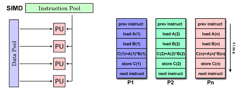
SIMD

• Single instruction stream Multiple Data stream
• Single instruction multiple data, parallel computer
• Each processing unit executes the same instruction in any clock cycle; Each processing unit can operate on different data elements
• It is suitable for dealing with problems with high regularity
• Synchronization and certainty
  

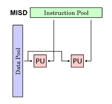
MISD

• Multiple instruction stream Single Data stream
• Multi instruction single data, parallel computer, there are few practical examples
• Each processing unit processes data through a separate instruction stream, and a single data stream is input to multiple processing units
  

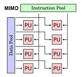
MIMD

• Multiple Instruction stream Single Data stream
• Multi instruction multi data, the most common parallel computer
• Each processing unit executes different instruction streams and uses different data streams
• Synchronous or asynchronous, deterministic or nondeterministic
  

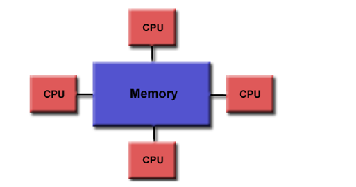
Shared memory

A storage structure of a parallel computer with a global address space

• characteristic
  All processors access all memory as a global address space
  Multiple processors run independently but share memory resources
  All processors can see the memory location change caused by one processor
• advantage
  The global address space is easy to program
  The memory is close to the CPU, and the data sharing between tasks is fast and uniform
• shortcoming
  Lack of scalability between memory and CPU
  High cost and high cost

They are classified as UMA and NUMA according to memory access time

UMA unified memory access

• Uniform Memory Access
• All processors have equal access to memory
• One processor updates the shared memory, which can be known by other processors, that is, cache coherence
  SMP, symmetric multi processing
  

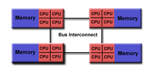
NUMA non-uniform memory access

• Non-Uniform Memory Access
• Connect multiple SMP S together by physical connection
• One SMP can access the memory of another SMP. Not all SMPS have equal access time to access all memory
• Slow memory access across links
• Cache coherence
  

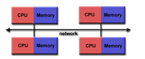
Distributed memory

A storage structure of parallel computer

• characteristic
  A communication network is required to connect the processor's memory
  The processor has local memory and there is no global address space
  Run independently, not applicable to cache coherence
  When the processor needs to access the data of other processors, the programmer needs to clearly define the data transmission mode and access time to synchronize the tasks
  The network structures used for data transmission vary greatly
  
• advantage
  Memory can increase as the number of processors increases
  Each processor can quickly access its own memory without conflict and overhead of maintaining cache consistency
  Low cost
• shortcoming
  Programmers need to be responsible for the details of many communications
  Because there is no global address space, it is difficult to establish distributed memory management mapping

Parallel computing model

PRAM

• Parallel Random Access Machine
• SIMD model of shared storage
  There is a centralized shared memory and an instruction controller to exchange data through the R/W of SM(Shared Memory) for implicit synchronous calculation.
• Concurrent read / write control strategy
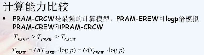
  According to the nature that the processor reads and writes to the shared storage unit at the same time, it is divided into
  
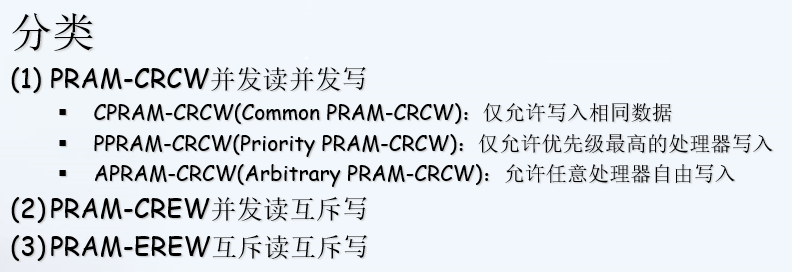
  (E:Exclusive C:Concurrent)
• Computing power of different concurrent read-write control strategies
  

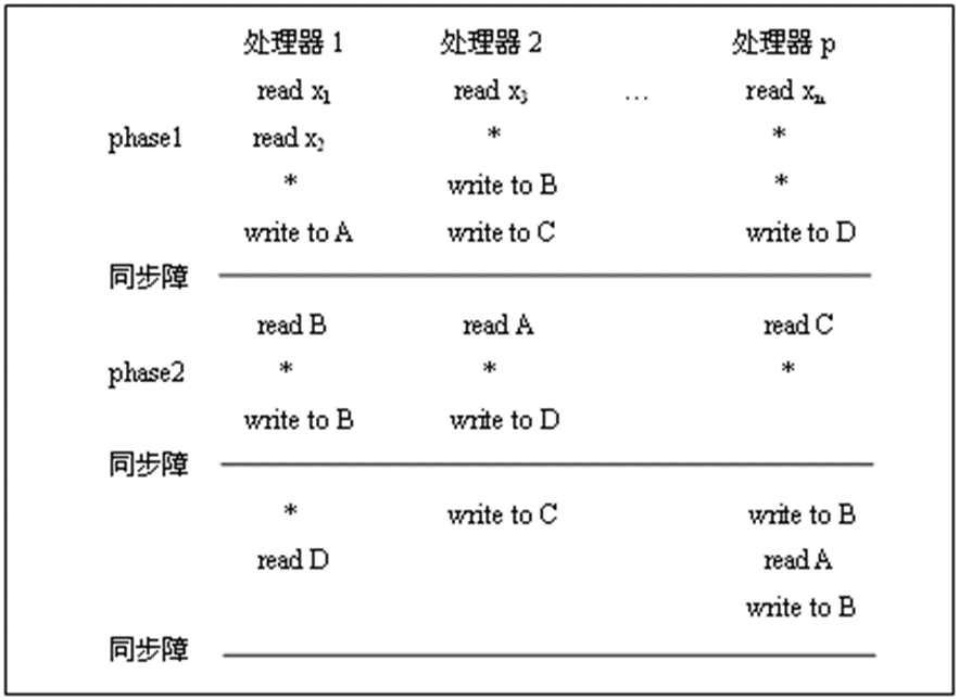
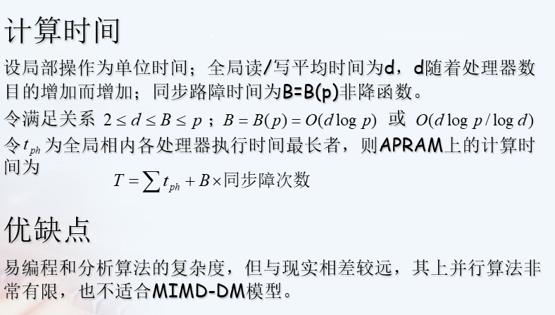
APRAM

• Asynchronous Parallel Access Machine, asynchronous PRAM model, also known as split phase PRAM
• For MIMD
  Each processor has its local memory, local clock and local program; There is no global clock, and each processor executes asynchronously; The processor communicates through SM; The dependencies between processors need to explicitly add synchronization roadblocks in parallel programs.
  
  

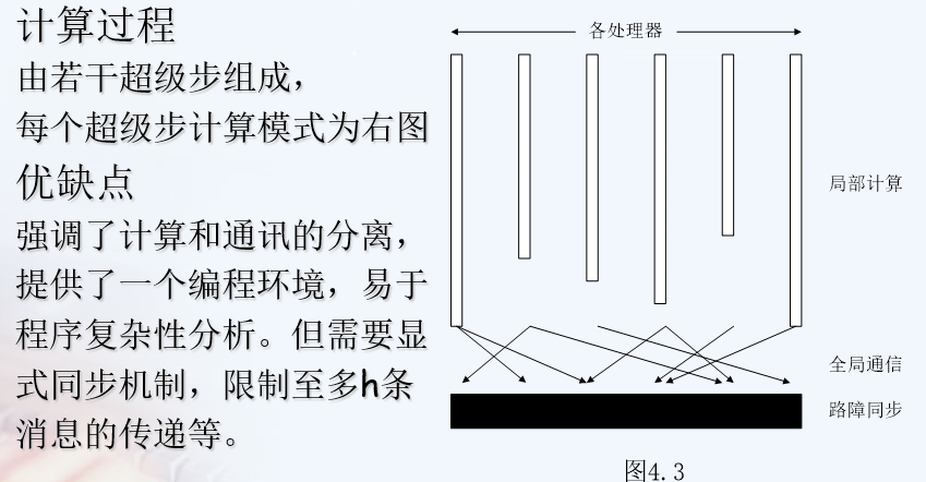
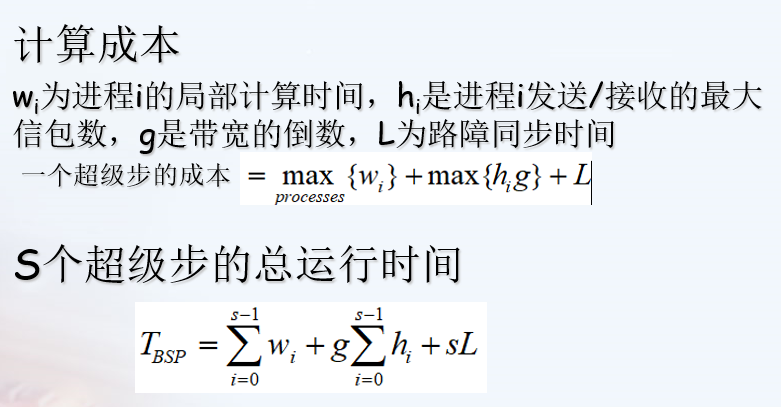
BSP

• Bulk Synchronous Parallel, a block synchronous model, is an asynchronous MIMD-DM(distributed memory) model
• Intra block asynchronous parallel, inter block explicit synchronization
  
  

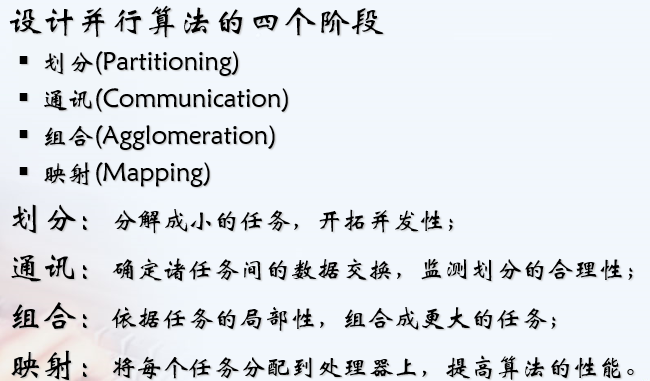
General design process of parallel method PCAM

• PCAM Partitioning Communication Agglomeration Mapping
• Partition communication combination mapping
  
  

MPI parallel programming

• Message Passing Interface
• Is a cross language parallel programming technology based on message passing, which supports point-to-point communication and broadcast communication. Message passing interface is a programming interface standard, not a detailed programming language. MPI is a standard or specification. At present, there are many implementations of MPI standards

Parallel test standard

Communication test standard

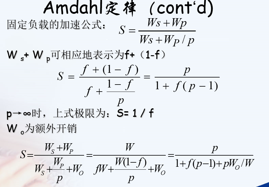
Amdahl's Law (fixed load)

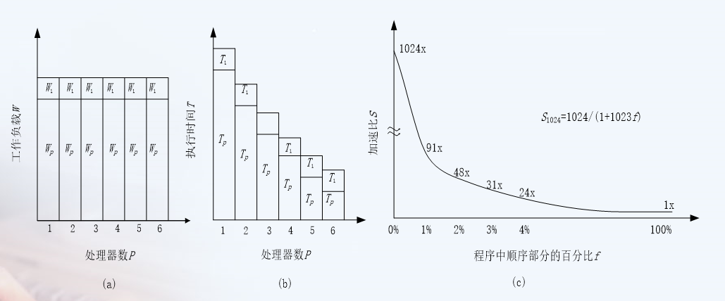
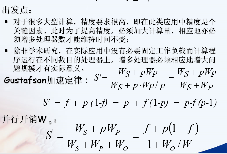
Gustafson's law

In practical problems, it is meaningless to increase the number of processors with a fixed load, so increasing the number of processors must also increase the load

Acceleration ratio and efficiency

Efficiency = S/P
Speedup ratio / number of processors
If the scale of the problem remains unchanged, the number of processors increases, and the efficiency decreases

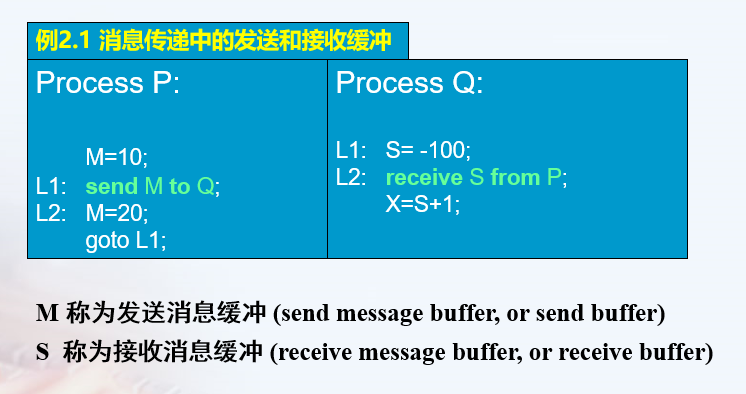
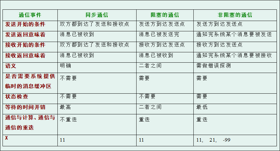
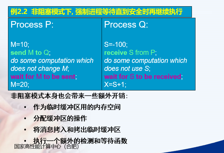
⭐⭐ There are three ways of message passing

Data sharing and process synchronization are realized between processes through message passing

• Synchronous messaging
  Synchronous Message Passing
  Start sending: both parties reach the sending point and the receiving point
  Send return and receive return: the message has been received
  Start receiving: both parties reach the sending point and the receiving point
  Waiting time: maximum
• Blocked messaging
  Blocking Message Passing
  Start sending: the sender reaches the sending point
  Send return: the message has been sent
  Start receiving: the receiver reaches the acceptance point
  Receive return: the message has been received
  Waiting time: between the two
• Non blocking messaging
  Nonblocking Message Passing
  Start sending: the sender reaches the sending point
  Send return: notify the system to send a message after sending
  Start receiving: the receiver reaches the acceptance point
  Receive return: notify the system to receive the message after receiving
  Waiting time: minimum

Similarities and differences of the three methods

MPI point-to-point communication and cluster communication

Point to point communication

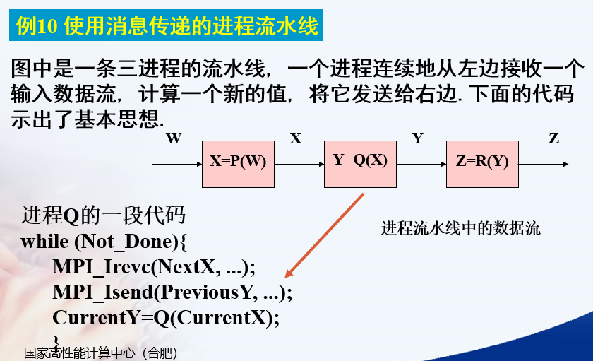
Q receives X for the next calculation
Q sends the last calculated Y
Then use the X received this time to calculate Y
The code in the figure below should be the process pipeline. How to receive and send specifically requires double buffering

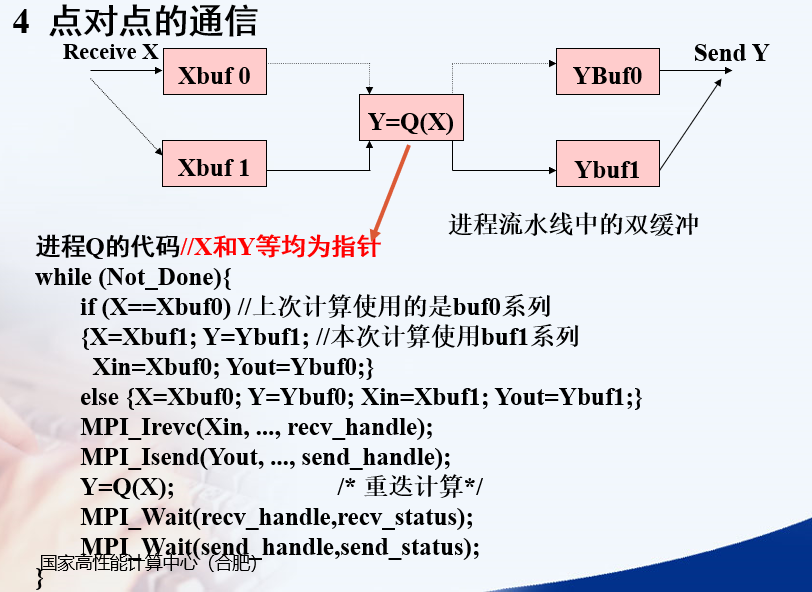
Isend and Irevc are non blocking. They return immediately after calling. It is necessary to call the waiting function
X Y Xbuf0 Xbuf1 Ybuf0 Ybuf1 Xin Yout are all pointers
Xin Yout is a pointer to the data to be sent or received
X Y refers to the buffer used for the current calculation

Cluster communication

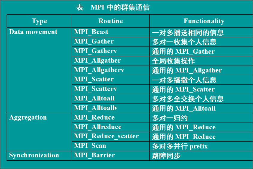
All processes in the communication subsystem must call the cluster routine

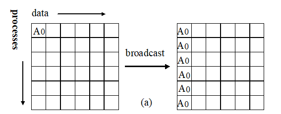
• Broadcast
  MPI_Bcast(Address, Count ,DataType, Root, Comm)
  The process marked as root sends the same message to all processes in the Comm communication subsystem
  
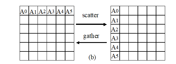
• Scatter Gather

MPI_Scatter(SendAddress, SendCount, SendDateTyoe, RecvAddress, RecvCount, RecvDataType, Root, Comm);
MPI_Gather(SendAddress, SendCount, SendDateTyoe, RecvAddress, RecvCount, RecvDataType, Root, Comm);

Broadcast: the root process sends a different message to each process, and the messages to be sent are orderly stored in the sending cache of the root process
Aggregation: root receives messages from each process, and the received messages are orderly stored in the receiving cache of root process.
Seeding and gathering are two opposite operations

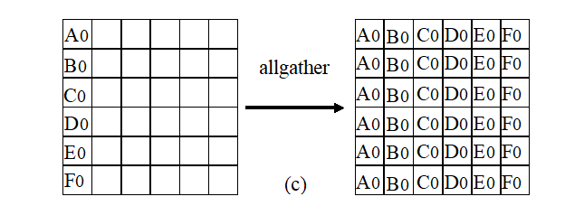
• Extended aggregation and dissemination (Allgather)

MPI_Allgather(SendAddress, SendCount, SendDateTyoe, RecvAddress, RecvCount, RecvDataType, Comm);

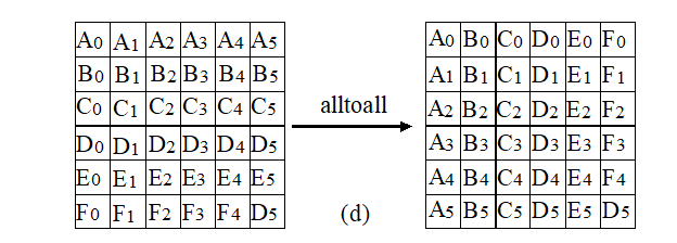
• Global exchange

MPI_Alltoall(SendAddress, SendCount, SendDateTyoe, RecvAddress, RecvCount, RecvDataType, Comm);

Each process sends messages to n processes, and the messages to be sent are orderly stored in the send cache
In other words, each process receives messages from n processes, and the messages to be received are orderly stored in the receive cache
Global exchange means that n processes gather n times. There are n^2 message communications in a global exchange

• Aggregation
  There are two aggregation operations: Reduction and Scan
  Reduction: each process stores the values to be reduced in SendAddress. All processes reduce these values into final results and store them in RecvAddress of the root process. The reduction operation is op

MPI_Reduce(SendAddress, RecvAddress, Count, DataType, Op, Root, Comm);

Scan: without root, combine some values into n final values and store them in RecvAddress of each process. The operation is op

MPI_Scan(SendAddress, RecvAddress, Count, DataType, Op, Comm);

• Barrier

MPI_Barrier(Comm);

All processes in the communication subsystem synchronize, that is, wait for each other until all processes finish executing their Barrier function

⭐⭐ Find the value of PI by MPI

#include <stdio.h>
#include <mpi.h>
#include <math.h>
long    n,    	/*number of slices         */
        i;    	/* slice counter           */
double sum, 	/* running sum             */
        pi,     /* approximate value of pi */
        mypi,
        x,      /* independent var.        */
        h;      /* base of slice           */
int group_size,my_rank;
 
main(argc,argv)
int argc;
char* argv[]; 
{      
	int group_size,my_rank;
	MPI_Status status;
	MPI_Init(&argc,&argv);
	MPI_Comm_rank( MPI_COMM_WORLD, &my_rank);
	MPI_Comm_size( MPI_COMM_WORLD, &group_size);
	 
	n=2000;
	/* Broadcast n to all other nodes */
	MPI_Bcast(&n,1,MPI_LONG,0,MPI_COMM_WORLD); 
	h = 1.0/(double) n;
	sum = 0.0;
	//Each process calculates a portion
	for (i = my_rank; i < n; i += group_size) {
		x = h*(i+0.5);
		sum = sum +4.0/(1.0+x*x);
	}
	mypi = h*sum;
	/*Global sum * reduce To the root process, the summation operation is used*/ 
	MPI_Reduce(&mypi,&pi,1,MPI_DOUBLE,MPI_SUM,0,MPI_COMM_WORLD); 
	if(my_rank==0) {        /* Node 0 handles output */
	printf("pi is approximately : %.16lf\n",pi);
	}
	MPI_Finalize();
}

MapReduce

Model principle

For big data that does not depend on each other, the best way to achieve parallelism is divide and conquer.
MPI and other parallel methods lack high-level parallel programming model, and programmers need to specify tasks such as storage, division and calculation; Without a unified parallel framework, programmers need to consider many details.
Therefore, MapReduce designs and provides a unified computing framework, hides most system layer details for programmers, and provides high-level concurrent programming model abstraction with Map and Reduce functions.

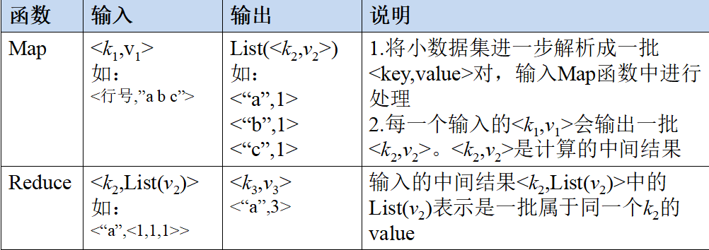
A large data set is divided into many independent splits, which are processed by multiple Map tasks in parallel
< K1, v1 >: K1 is the primary key and v1 is the data. After Map processing, many intermediate results are generated, that is, list (< K2, V2 >).
Reduce merges the intermediate results, merges the data with equal key values, i.e. < K2, list (V2) >, and finally generates the final result, i.e. < K3, V3 >

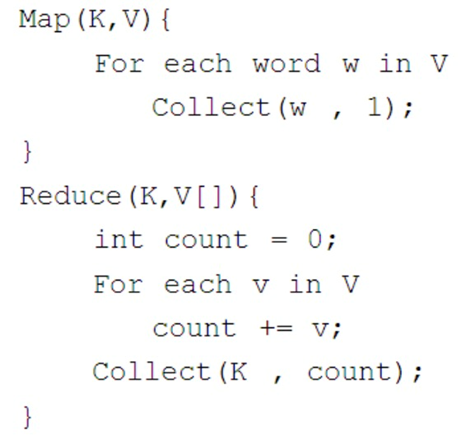
⭐⭐ wordcount instance

Illustration:

Core pseudo code:

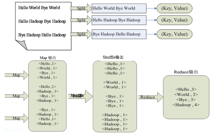
Click to view the pseudo code

public class Mapper()
{
	/*
	key And value are the key value pairs entered
	context Is the result of the output
	*/
	public void map(Object key, Text value, Context context)
				throws IOException, InterruptedException {
		//By default, the data of each row is taken. Each row has spaces and is divided by spaces
		String lineContent = value.toString();	//Take out the data of each row
		String words[] = lineContent.split(" ");	//Split each row of data
		
		for(String word : words){	//Loop each word and then generate data
				//The number of saved words finally generated for each word is 1
				context.write(word, 1);
		}
	}	
}

public class Reducer()
{
	/*
	key And values are intermediate results of map output, which need to be processed by reduce
	context This is the final result of reducer output
	*/	
	public void reduce(Text key, Iterable<IntWritable> values, Context context)
			throws IOException, InterruptedException {{
		int sum = 0 ;	//Save the total number of occurrences of each word
	}
	for(IntWritable count :  values){
		sum += count.get();
	}
	context.write(key, sum);
}

public static void main(String[] args) throws Exception{
	//Make relevant configuration
	Configuration configuration=new Configuration();
	//Create a work object
	Job job=Job.getInstance(configuration);
	//Set current work object
	job.setJarByClass(Myjob.class);
	//Set map object class
	job.setMapperClass(Mapper.class);
	//Set the reduce object class
	job.setReducerClass(Reducer.class);
	//Set the key type of the output
	job.setOutputKeyClass(Text.class);
	//Set the value type of the output
	job.setOutputValueClass(IntWritable.class);
	//Set the location of the imported file
	FileInputFormat.addInputPath(job, new Path("/hadoop/hadoop.txt"));
	//Set file location for output
	FileOutputFormat.setOutputPath(job, new Path("/hadoop/out"));
	job.waitForCompletion(true);
	return 0;
}

Fault tolerant control strategy (4 kinds)

Fault tolerance: the system can continue to provide services under the premise of failure

Checkpoint fault tolerance

Process: periodic backup and rollback recovery
When a task fails, the calculation can be resumed from the last successful checkpoint

Backup overhead and recovery efficiency cannot be combined

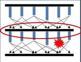
Lineage fault tolerance

Dependency of input and output:
Narrow dependence: one to one
Wide dependence: one to many

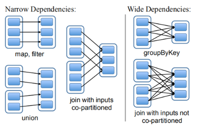
Lineage fault tolerance: record the dependency of intermediate results, recalculate a part according to the lineage information, and recover the lost data
If the lineage information is too long, the calculation will be time-consuming, and checkpoints need to be used to avoid too many repeated calculations

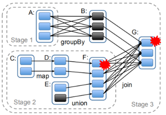
Recalculating F1 with D1 can accurately recover data, but it is only effective for narrow dependencies

Speculative execution

If a task is executed too slowly, a backup task will be started. Finally, the results of the faster tasks in the original task and the backup task will be used.
Speculative execution is turned off by default, because repeated tasks will reduce the efficiency of the cluster.
Speculative execution is space for time. It is generally started when resources are idle and job completion is large

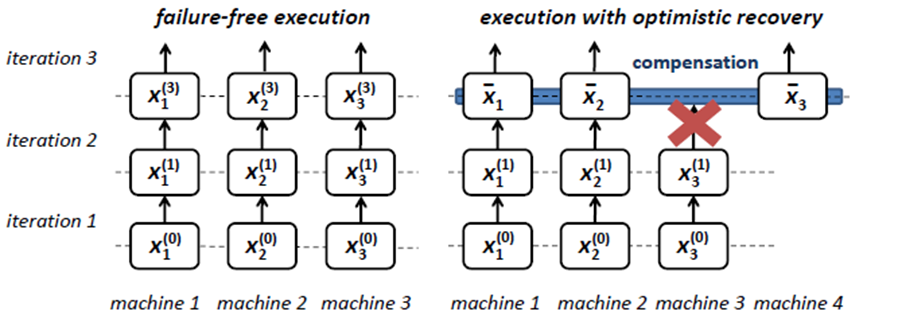
Compensated fault tolerance

No preparation, reset lost data in case of failure (recalculation)
Advantages: no redundancy (the first three have redundancy, data redundancy or computational redundancy)
Disadvantages: it has great limitations and is only applicable to some algorithms

Note: please point out any errors!