I Mean RFM model algorithm
Read the corresponding data from the csv file

data=pd.read_csv('./dataset.csv',encoding='ISO-8859-1')

#Read customer information in 2014

data_14=data[data['Order-year']==2014]
data_14

2. Get the corresponding column

data_14 = data_14[['CustomerID','OrderDate','Sales']]
data_14 

CustomerID is the user id
OrderDate is the order date
Sales is the sales amount

3. Copy data (to avoid changing the original data when modifying)

customerdf=data_14.copy()
customerdf

4. Set CustomerID as index

customerdf.set_index('CustomerID',drop=True,inplace=True)

5 add transaction times field (convenient for later calculation of F)

customerdf['orders']=1
customerdf

6. Make a pivot table
Last purchase time purchase times total purchase amount

rfmdf=customerdf.pivot_table(
    index=['CustomerID'],
    values=['OrderDate','orders','Sales'],
    aggfunc={
        'OrderDate':'max',
        'orders':'sum',
        'Sales':'sum'
    }
)

aggfunc calculates the maximum value of OrderDate for the setting of each field, orders is the sum of the number of orders, and Sales is the total Sales amount of each user
7. R F M of each user
R can be calculated by subtracting the last purchase time of each user from the same standard. If the standard is the same, the R standard is the same

rfmdf['R']=(rfmdf.OrderDate.max()-rfmdf.OrderDate).dt.days
rfmdf.rename(columns={'Sales':'M','orders':'F'},inplace=True)
rfmdf

rfmdf.OrderDate.max() is the maximum value of the order placing date in the whole year of 2014. This value can be selected arbitrarily. If a value is selected, the calculated value of each column is the standard value
8 user labeling algorithm

Judgment result return string.So that it can be spliced later,Integer numbers cannot be spliced
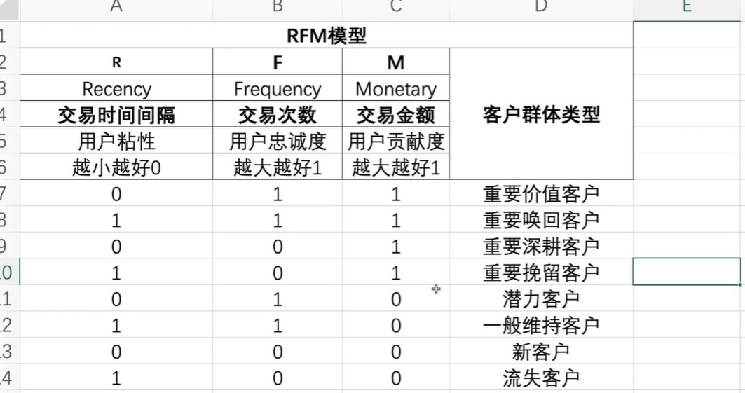
def rfm_func(x):
#The difference from the mean value is set to 0 and 1
    res=x.apply(lambda x:'1'if x>0 else '0')
    label=res.R+res.F+res.M
    d={
        '011':'Important value customers', 
        '111':'Important call back customers',
        '001':'Important deep ploughing customers',
        '101':'Important retention customers',
        '010':'Potential customers',
        '110':'General maintenance customer',
        '000':'New customers',
        '100':'Lost customers'
    }
    result=d[label]
    return result

9. Connect RFMS, make difference between the average value of each RFM, and then label each user with a function

rfmdf['label']=rfmdf[['R','F','M']].apply(lambda x:x-x.mean()).apply(rfm_func,axis=1)

10. Calculate the number of each customer type

rfmdf.groupby('label').count()

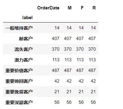
11. Plot each customer type as abscissa and the value of customer type, i.e. quantity, as ordinate

rfmdf.label.value_counts().plot.bar(figsize=(20,8),fontsize=15)

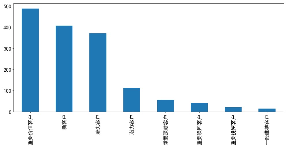
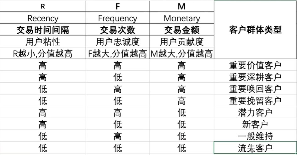
II. RFM scoring algorithm
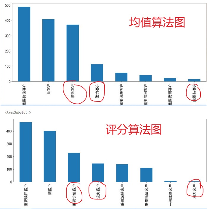
Note: the mean value algorithm reduces the error of the maximum and minimum values, so that the whole statistical error becomes larger
The scoring algorithm is to score each user according to a certain interval, so as to improve the overall statistical accuracy

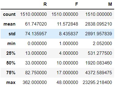
1. Basic information of statistical table

customer_grade_df = rfmdf[['R','F','M']]
customer_grade_df.describe()

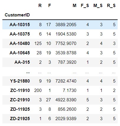
2. Set scoring range

#1.1 score the range of F value. The larger the F value, the higher the score
section_list_F=[0,5,10,15,20,50]
grade_F=pd.cut(customer_grade_df['F'],bins=section_list_F,labels=[1,2,3,4,5])
grade_F
customer_grade_df['F_S']=grade_F.values
#1.2 score the range of M value. The larger the M value, the higher the score
section_list_M=[0,500,1000,5000,10000,30000]
grade_M=pd.cut(customer_grade_df['M'],bins=section_list_M,labels=[1,2,3,4,5])
grade_M
customer_grade_df['M_S']=grade_M.values
#1.3 score the range of R value. The smaller the R value, the higher the score
section_list_R=[-1,32,93,186,270,365]
grade_R=pd.cut(customer_grade_df['R'],bins=section_list_R,labels=[5,4,3,2,1])
grade_R
customer_grade_df['R_S']=grade_R.values
customer_grade_df

Note: the interval of each RFM is set according to the maximum and minimum values in the above table. Be sure to include the values of the field, otherwise the whole statistical value will be error

3. View the basic information of the table

customer_grade_df.describe()
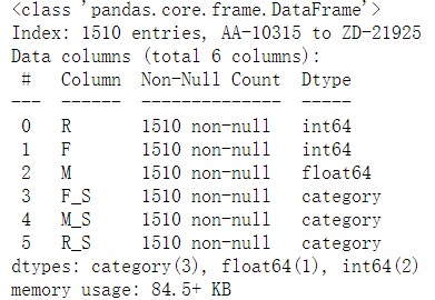
#You can find R_S,F_S,M_S is not a floating point number, but a category type 
#Calculation cannot be performed and conversion is required. This is caused by the cut function of pandas library
customer_grade_df.info()  

4. Modify the category type to int64

rfm_score_grade=pd.DataFrame(customer_grade_df[['R_S','F_S','M_S']],dtype=np.int64)
rfm_score_grade.dtypes

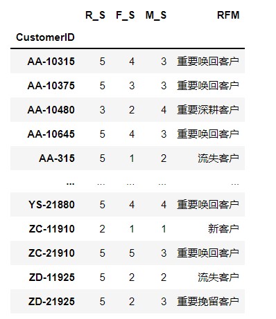
5. Label the user according to the scoring situation (the same as the mean algorithm)

def rfm_score_func(x):
    level=x.apply(lambda x: '1'if x>=0 else '0')
    label = level.R_S+level.F_S+level.M_S
    d={
        '011':'Important value customers', 
        '111':'Important call back customers',
        '001':'Important deep ploughing customers',
        '101':'Important retention customers',
        '010':'Potential customers',
        '110':'General maintenance customer',
        '000':'New customers',
        '100':'Lost customers'
    }
    result=d[label]
    return result
rfm_score_grade['RFM']=rfm_score_grade[['R_S','F_S','M_S']].apply(lambda x:x-x.mean()).apply(rfm_score_func,axis=1 )
rfm_score_grade

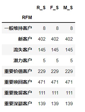
6. Calculate the number of customers of each type

rfm_score_grade.groupby('RFM').count()

7. Drawing

rfm_score_grade.RFM.value_counts().plot.bar(figsize=(20,8),fontsize=16)

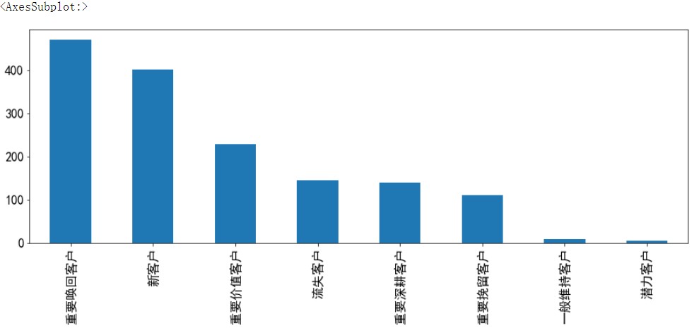
Three analogy mean algorithm chart and scoring algorithm chart, it can be seen that the mean error is large