1. Ridge regression model

1.1 background

For regression problems, their basic contents are basically the same, so ridge regression model and linear regression model similar:
y = θ 0 x 0 + θ 1 x 1 + θ 2 x 2 + . . . θ n x n {\color{Violet}y = θ_{0}x_{0}+θ_{1}x_{1}+θ_{2}x_{2}+...θ_{n}x_{n}} y= θ 0​x0​+ θ 1​x1​+ θ 2​x2​+... θ The difference between them is mainly reflected in the construction of loss function.

For some matrices, a small change of an element in the matrix will cause a large error in the final calculation result. This kind of matrix is called "ill conditioned matrix". Sometimes incorrect calculation methods will also make a normal matrix ill conditioned in operation. For Gaussian elimination method, if the elements on the principal element (i.e. the elements on the diagonal) are very small, it will show ill conditioned characteristics in calculation.

The ridge regression model uses the improved least square estimation method. By abandoning the unbiased nature of the least square method, the regression coefficient is obtained at the cost of losing some information and reducing accuracy. It is a more practical and reliable regression method, and the fitting of ill conditioned data is better than the least square method.

1.2 loss function

The loss function of ridge regression model is constructed as follows:
J ( θ ) = 1 2 m ∑ i = 1 m ( y i − w x i ) 2 + λ 2 ∑ j = 1 n θ j 2 {\color{Violet}J(\theta) = \frac{1}{2m}\sum_{i=1}^{m}(y_{i}-wx_{i})^{2}+\frac{\lambda}{2}\sum_{j=1}^{n}\theta_{j}^{2}} J(θ)=2m1​i=1∑m​(yi​−wxi​)2+2λ​j=1∑n​θj2​

In the above formula 𝑤 {\color{Red}𝑤} w is the length 𝑛 {\color{Red}𝑛} The vector of n, excluding the coefficients of the intercept term θ 0 {\color{Red}θ_{0}} θ0​ . m {\color{Red}m} m is the number of samples; 𝑛 {\color{Red}𝑛} n is the characteristic number. Similarly, the matrix can be used to simplify the expression, and the results are as follows:
J ( θ ) = 1 2 ( Y − Y ^ ) 2 + λ 2 θ 2 {\color{Violet}J(\theta)=\frac{1}{2}(Y-\hat Y)^{2}+\frac{\lambda}{2}\theta ^{2}} J(θ)=21​(Y−Y^)2+2λ​θ2

Let's face up θ {\color{Red}\theta} θ The optimal solution can be obtained by making the derivative equal to 0, and the optimal solution can be obtained after conversion θ {\color{Red}\theta} θ The expression is:
θ = ( X T X + λ I ) − 1 ( X T Y ) {\color{Violet}\theta = (X^{T}X+\lambda I)^{-1}(X^{T}Y)} θ=(XTX+λI)−1(XTY)

among λ {\color{Red}\lambda} λ As an incoming parameter, we need to set its value, and I {\color{Red}I} I is the identity matrix. Compared with the linear regression model, this model adds λ I {\color{Red}\lambda I} λ I this one, this can guarantee X T X {\color{Red}X^{T}X} XTX is reversible, so it can solve the problem of ill conditioned matrix in general.

2. Relevant codes

2.1 ridgeregression class

import numpy as np
#Define RidgeRegression
class RidgeRegression :
    def __init__(self):
        '''Initialize the linear regression model, and finally get theta'''
        self.theta = None
        
    # Implemented by code θ Enter the values of X and y, which can be specified λ The default is 0.2    
    def fit(self,xMat,yMat,lam=0.2):
        xMat=np.mat(xMat)#Convert data to matrix
        yMat=np.mat(yMat).T#Convert the data into a matrix and transpose it
        xTx = xMat.T*xMat#Matrix xMat transposed and multiplied
        denom = xTx + np.eye(np.shape(xMat)[1])*lam#Formula XTX+ λ Representation code of I
        # Judge whether denom is strange
        if np.linalg.det(denom) == 0.0:
            print("This matrix is singular and cannot be inversed")
            return
        self.theta = denom.I * (xMat.T*yMat)#According to the optimal solution formula θ value

    # Predict the test data and enter the test_data is the original X. we need to use theta to get the corresponding predicted value
    def predict(self,test_data):
        test_data=np.mat(test_data)#Convert data to matrix
        y_predict=test_data*self.theta#Obtained by θ Value to predict the data
        
        return y_predict

2.2 solution code

import pandas as pd
import numpy as np
#Read data
data = pd.read_csv('/data/shixunfiles/11996b194a005626887e927dd336f390_1577324743961.csv')

#Extract eigenvalues and real values
X = data.iloc[:,:-1].values
y = data.iloc[:,-1].values

#Add a column x0 to the characteristic value, and all values of x0 are 1
X = np.hstack((np.ones((X.shape[0],1)),X))

#Establish the model and train the model
rr = RidgeRegression()
rr.fit(X,y)

#The data is predicted. In order to find the fitting curve, the original data is used for prediction
ypredict = rr.predict(X)

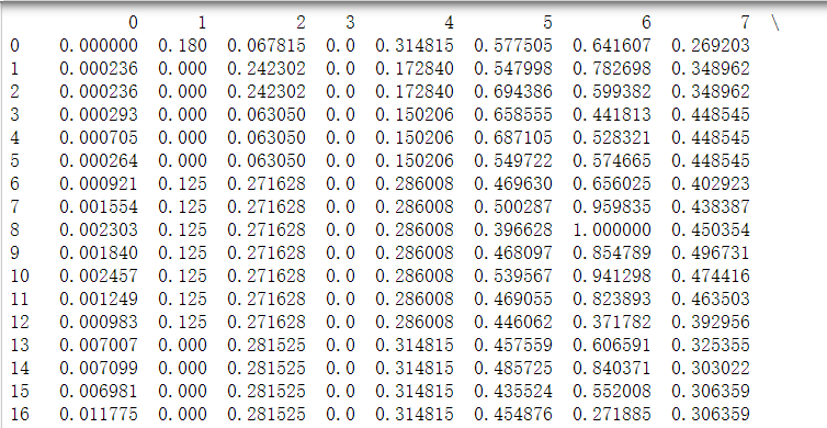
Here are some data in csv. The column with subscript 0-6 represents the eigenvalue of each feature point, and the column with subscript 7 represents the corresponding label of each feature point. Note that we need to add a column x0 with values of 1.

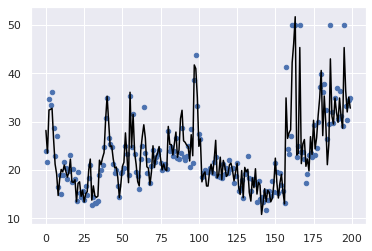
2.3 drawing code

import matplotlib.pyplot as plt
import seaborn as sns;
sns.set()
#Select 200 pieces of data to view
plt.scatter(range(200),y[:200],s=20)
plt.plot(range(200),ypredict[:200],color='black')