01. Preface
In the near future, it is expected that the emerging digital gene expression (DGE) technology will surpass microarray technology in many applications of functional genomics. One of the basic data analysis tasks, especially gene expression research, involves determining whether there is evidence that transcripts or exons are significantly different in the experiment.
edgeR is the differential expression of repeat count data of Bioconductor software package used for inspection. The over dispersed Poisson model is used to explain biological and technological variability. Empirical Bayesian method is used to adjust the excessive dispersion of degrees across transcripts and improve the reliability of reasoning. The method can even use the minimum replication level to provide that at least one phenotype or experimental condition is replicated. The software may have other applications beyond sequencing data, such as proteomic peptide count data.
This article continues to show the differential gene analysis process of R-package edgeR. Similar to limma, DESeq2 and edgeR, which are widely used r packages, we can often see them in the literature. Based on the quantitative expression values obtained by transcriptome sequencing, there are many methods to identify genes or other non coding RNA molecules with differential expression changes.
02. Data file reading
We still use the data set of TCGA-COAD for data reading. We mentioned the reading of expression data and the acquisition of clinical information grouping in the previous issue, but the source code is attached here to facilitate a comprehensive understanding of the overall analysis, as follows:
library(TCGAbiolinks)
query <- GDCquery(project ="TCGA-COAD",
                  data.category = "Transcriptome Profiling",
                  data.type ="Gene Expression Quantification" ,
                  workflow.type="HTSeq - Counts")
                  samplesDown <- getResults(query,cols=c("cases"))

dataSmTP <- TCGAquery_SampleTypes(barcode = samplesDown,
                                  typesample = "TP")

dataSmNT <- TCGAquery_SampleTypes(barcode = samplesDown,
                                  typesample = "NT")

group<-as.data.frame(list(Sample=c(dataSmTP,dataSmNT),
     Group=c(rep("TP",length(dataSmTP)),rep("NT",length(dataSmNT)))))

###Set the barcodes parameter
queryDown <- GDCquery(project = "TCGA-COAD",
                      data.category = "Transcriptome Profiling",
                      data.type = "Gene Expression Quantification",
                      workflow.type = "HTSeq - Counts",
                      barcode = c(dataSmTP, dataSmNT))

# The data downloaded for the first time needs to be executed. It has been downloaded here and is not executed. The default storage location is in the GDCdata folder under the current working directory.
#GDCdownload(queryDown,method = "api",
#            directory = "GDCdata",
 #           files.per.chunk = 10)

# GDCprepare():Prepare GDC data to prepare GDC data for analysis in R language
dataPrep1 <- GDCprepare(query = queryDown,
                        save = TRUE,
                        save.filename = "COAD_case.rda")

# Function Description: array intensity correlation (AAIC) and correlation boxplot to define outlier

dataPrep2 <- TCGAanalyze_Preprocessing(object = dataPrep1,
                                       cor.cut = 0.6,
                                       datatype = "HTSeq - Counts")
dim(dataPrep2)
03. Data preprocessing
In the data processing part, we use edgeR's data filtering mode. The article refers to filtering low count data, such as CPM Standardization (recommended), and then standardization. Take TMM standardization as an example, as follows:
library(edgeR)
#(1) Build table
dgelist <- DGEList(counts = dataPrep2, group = group$Group)

#(2) Filter
keep <- rowSums(cpm(dgelist) > 1 ) >= 2
dgelist <- dgelist[keep, , keep.lib.sizes = FALSE]

#(3) Standardization
dgelist_norm <- calcNormFactors(dgelist, method = 'TMM')
04. Differential expression analysis
Firstly, the experimental design matrix is constructed according to the grouping information. In the grouping information, the control group must be in the front and the processing group must be in the back. Then) estimate the dispersion of gene expression value and model fitting. edgeR provides two fitting algorithms, including:
-
Negative binomial generalized log linear model;
-
Quasi Likelihood negative binomial generalized log linear model.
design <- model.matrix(~group$Group)

#install.packages("statmod")
library(statmod)
dge <- estimateDisp(dgelist_norm, design, robust = TRUE)

#(2) For model fitting, edgeR provides a variety of fitting algorithms
#Negative binomial generalized log linear model
fit1 <- glmFit(dge, design, robust = TRUE)
lrt1 <- topTags(glmLRT(fit1), n = nrow(dgelist$counts))
lrt1<-as.data.frame(lrt1)
head(lrt1)

##                     logFC      logCPM        LR        PValue           FDR
## ENSG00000142959 -5.924830  3.20085238 1457.1137 8.159939e-319 2.592984e-314
## ENSG00000163815 -4.223787  2.59792097 1145.7948 3.679815e-251 5.846674e-247
## ENSG00000107611 -5.131288  1.71477711 1122.0643 5.289173e-246 5.602468e-242
## ENSG00000162461 -4.101967  1.51480635 1085.9423 3.752089e-238 2.980753e-234
## ENSG00000163959 -4.295806  3.39558390 1080.7407 5.067873e-237 3.220836e-233
## ENSG00000144410 -6.284258 -0.02616284  916.3497 2.739233e-201 1.450744e-197

#Quasi Likelihood negative binomial generalized log linear model
fit2 <- glmQLFit(dge, design, robust = TRUE)
lrt2 <- topTags(glmQLFTest(fit2), n = nrow(dgelist$counts))
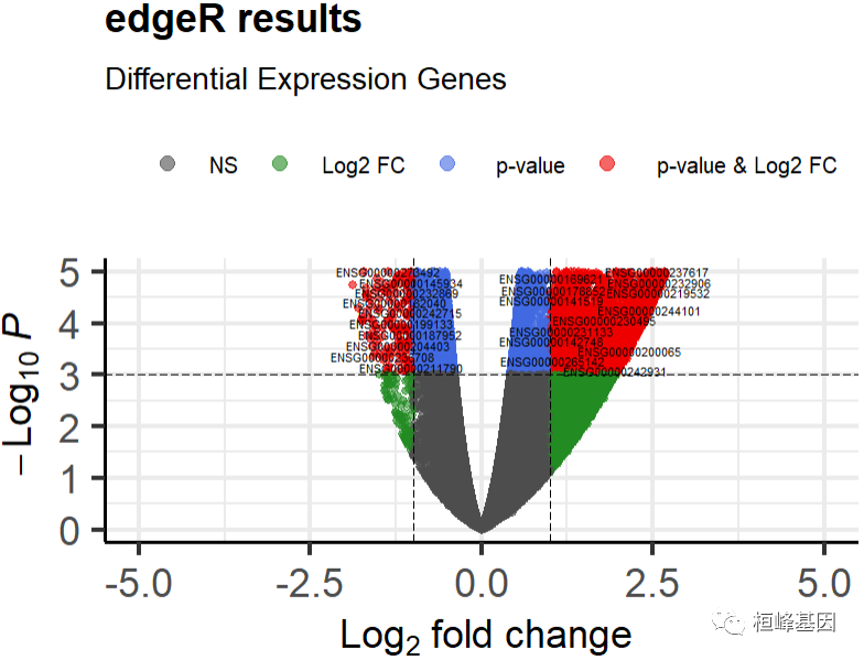
05. Map volcanoes
The enhanced volcano package is still used for the drawing of the volcano map, because it is very easy to use. Only a few parameters need to be modified, such as the variables of the input matrix and the column names used by the x and y variables to output the volcano map. Here we use the differential gene results obtained by the negative binomial generalized log linear model, as follows:
require(EnhancedVolcano)
EnhancedVolcano(lrt1,
                lab = rownames(lrt1),
                labSize = 2,
                x = "logFC",
                y = "PValue",
                #selectLab = rownames(lrt)[1:4],
                xlab = bquote(~Log[2]~ "fold change"),
                ylab = bquote(~-Log[10]~italic(P)),
                pCutoff = 0.001,## pvalue valve?
                FCcutoff = 1,## FC cutoff
                xlim = c(-5,5),
                ylim = c(0,5),
                colAlpha = 0.6,
                legendLabels =c("NS","Log2 FC"," p-value",
                                " p-value & Log2 FC"),
                legendPosition = "top",
                legendLabSize = 10,
                legendIconSize = 3.0,
                pointSize = 1.5,
                title ="edgeR results",
                subtitle = 'Differential Expression Genes',
)
06. Screening differential genes
To screen differential genes, first arrange the table in ascending order according to FDR value, continue to sort in descending order according to log2FC under the same FDR value, and then mark the genes in three cases:
-
up regulated genes: log2FC ≥ 1 & FDR < 0.01;
-
down regulated genes: log2FC ≤ - 1 & FDR < 0.01;
-
Non differential genes: the rest mark none.
lrt1 <- lrt1[order(lrt1$FDR, lrt1$logFC, decreasing = c(FALSE, TRUE)), ]

lrt1[which(lrt1$logFC >= 1 & lrt1$FDR < 0.01),'sig'] <- 'up'
lrt1[which(lrt1$logFC <= -1 & lrt1$FDR < 0.01),'sig'] <- 'down'
lrt1[which(abs(lrt1$logFC) <= 1 | lrt1$FDR >= 0.01),'sig'] <- 'none'
#Summary of differentially selected genes
res <- subset(lrt1, sig %in% c('up', 'down'))
head(res)

##                     logFC      logCPM        LR        PValue           FDR  sig
## ENSG00000142959 -5.924830  3.20085238 1457.1137 8.159939e-319 2.592984e-314 down
## ENSG00000163815 -4.223787  2.59792097 1145.7948 3.679815e-251 5.846674e-247 down
## ENSG00000107611 -5.131288  1.71477711 1122.0643 5.289173e-246 5.602468e-242 down
## ENSG00000162461 -4.101967  1.51480635 1085.9423 3.752089e-238 2.980753e-234 down
## ENSG00000163959 -4.295806  3.39558390 1080.7407 5.067873e-237 3.220836e-233 down
## ENSG00000144410 -6.284258 -0.02616284  916.3497 2.739233e-201 1.450744e-197 down
The number of differential genes is still quite large. It is estimated that the data volume of normal samples is very small, resulting in very high bias.
table(res$sig)
##
## down   up
## 3308 8164
Three software packages based on gene expression, limma, DESeq2 and edgeR, have been introduced. Filter your own data and use it. Later, we will talk about how to display the differentially expressed data in SCI articles. Please look forward to it!
Pay attention to the official account, update every day!

Huanfeng gene
Bioinformatics analysis, SCI article writing and bioinformatics basic knowledge learning: R language learning, perl basic programming, linux system commands, Python meet you better
40 original content
official account
Reference:
-
Robinson MD, McCarthy DJ, Smyth GK. edgeR: a Bioconductor package for differential expression analysis of digital gene expression data. Bioinformatics. 2010;26(1):139-140.
-
Agarwal A, Koppstein D, Rozowsky J, et al. Comparison and calibration of transcriptome data from RNA-Seq and tiling arrays. BMC Genomics. 2010;11:383.
-
Love MI, Huber W, Anders S. Moderated estimation of fold change and dispersion for RNA-seq data with DESeq2. Genome Biol. 2014;15(12):550.
-
Maurya NS, Kushwaha S, Chawade A, Mani A. Transcriptome profiling by combined machine learning and statistical R analysis identifies TMEM236 as a potential novel diagnostic biomarker for colorectal cancer. Sci Rep. 2021;11(1):14304.